Overview
Presentation & objectives
This page contains a tutorial about the class prerequisites. It serves 2 objectives. It is both:
- a refresher on some basic R programming, in particular:
- control structures (
if/elsestatement,forloop) - functions
- variable assignation
- vector manipulation
- control structures (
- a refresher on likelihood modeling and maximum likelihood estimation
Disclaimer: those concepts are only covered on a superficial level, just enough so that your memory and technical skills are fresh for the start of the class.
Instructions
First, read through the 3 sections Motivating data example, Maximum Likelihood Estimation (MLE) refresher & R programming refresher.
Second, do the 2 practicals, one for each model. In each practical, you have 3 levels of difficulties, feel free to use the one that best suits your abilities (from hardest to easiest):
- Minimum help: most of the code you are expected to produce to answer questions is hidden. In this level, you need to do most of the thinking by yourself.
- Intermediate help: unfold the partial code by clicking on the
Show intermediate help button. You will then be provided with the minimal structure of the expected code to produce, allowing you to focus on the technical aspects without the added code design overhead. - Full help solutions: you can find the full solution for these practicals here.
Use this as a last resort, for questions where you have tried the intermediate help level first ! You will then only need to copy and paste the code for executing the solutions: learning this way is harder and less effective, unless you have first thought about a solution for a few minutes.
Motivating data example
We will use data from a randomized clinical trial by Goldman et al. (1996)1 comparing the efficacy of 2 different antiretroviral drugs (namely didanosine and zalcitabine) in 467 HIV infected patients intolerant or failing to zidovudine (“AZT”) between 1990 and 1992. Three observed variables are available to us from the goldman1996.csv file (download here ):
AIDS: AIDS status (1AIDS,0no AIDS)CD4: CD4 cell count in cell/mm3CD4t: transformed CD4 cell count (CD41/4)
Below is a quantitative summary of the characteristics of those 3 observed variables.
| Variable | N = 4671 |
|---|---|
| AIDS | 307 (66%) |
| CD4 | 37 (11, 109) |
| CD4t | 2.47 (1.82, 3.23) |
| 1 Median (IQR) or n (%) | |
We will use 2 illustrating use-cases:
- Bernoulli modeling of the AIDS status
- Gaussian linear regression applied to the (transformed) CD4 count depending on the AIDS status
Maximum Likelihood Estimation (MLE) refresher
In statistics, the likelihood refers to the product of the density function of a specific modeling distribution (chosen by the modeler) evaluated at each observation, given a set of parameter values.
In inferential statistics, the scientific question of interest can often be formulated with respect to the value of those parameters from the modeling distribution. In other words, the question is often about the value of a specific parameter (e.g. the mean). To estimate those values using an observed sample from the population of interest, the Maximum Likelihood approach is very powerful: the idea is to find the parameter values that will maximize the likelihood of the observations.
As long as the number of parameter remains relatively small compared to the number of available observations, numerical optimization should be able to identify the (at least local) maximum for the likelihood parameters, providing a Maximum Likelihood Estimation (MLE) of those parameters. Below are 2 graphics illustrating the MLE for a simple Bernoulli model of the AIDS status in the Goldman et al. dataset, parameterized by \(\theta\) as the probability of having AIDS.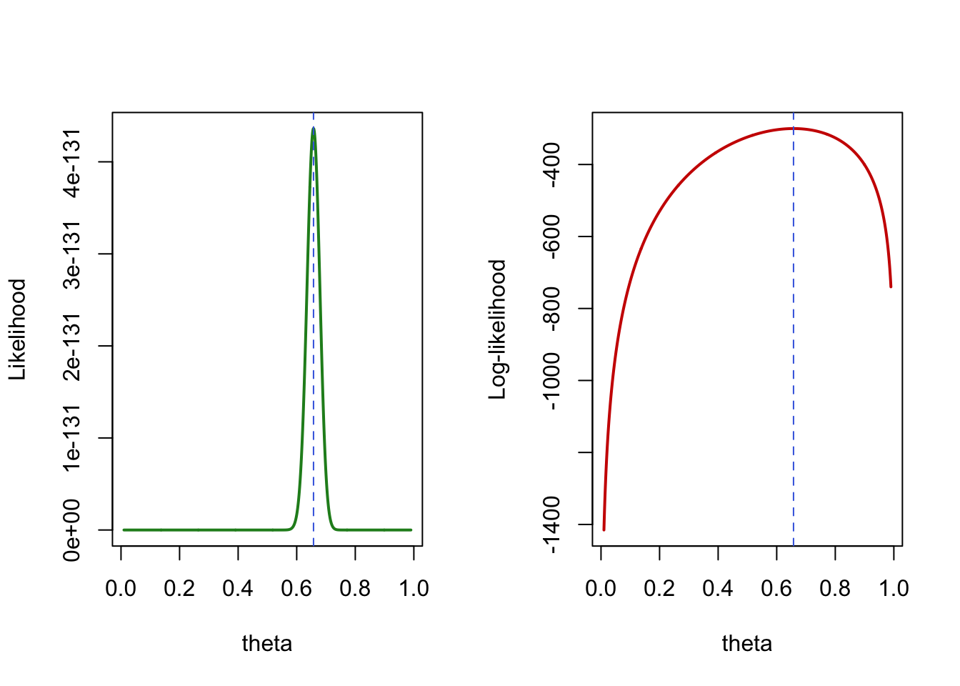
Figure 1: MLE illustration for a Bernoulli likelihood of the AIDS status in Goldman et al. dataset.
For a short informal introduction to those concept, one can watch the StatQuest video below:
R programming refresher
Variable name assignment
In R if you want to store values and objects for later use in a code, you need to assign it to a reference name. This can be done through the arrow operator: <- .
Two examples below:
a <- 2
a
## [1] 2
b <- "value"
b
## [1] "value"Unlike those examples, it is always preferable to use meaningful names, so that your code is easy to read and understand (there is a reasonable chance that at least 1 person – i.e. future you – will read your code one day). Spoiler alert: this is hard !
For a more advanced and precise presentation of Values and name assignment in R, you can have a look at the 2nd chapter of Advanced R by Wickham (2019) (freely available online).
Vector types and vector manipulation
There actually are two sorts of vectors in R atomic vectors and lists. The main difference is that atomic vectors are homogeneous in type (e.g. double, character, logical…), while list can be heterogeneous.
In R, vectors are indexed from 1 to the their length(). They can be subset using the [ operator, and list elements can be accessed thanks to the [[ operator. See the examples below:
v <- c(45.2, 77.1, 34.8)
v[1]
v[2]
v[2:3]
## [1] 45.2
## [1] 77.1
## [1] 77.1 34.8
l <- list("a", FALSE, 2)
l[[3]]
l[3]
l[2:3]
## [1] 2
## [[1]]
## [1] 2
##
## [[1]]
## [1] FALSE
##
## [[2]]
## [1] 2
For a longer presentation of vectors in R, you can have a look at the 20th chapter of R for Data Science by Wickham and Grolemund (2016) (freely available online). For a more advanced and precise presentation of vectors in R, you can have a look at the 3rd chapter of Advanced R by Wickham (2019) (freely available online).
Functions
The primary value of using functions is to make your code easier to read, understand and debug. This suppose the use of human-friendly names (cf. Variable assignation sub-section above).
Why write functions ? To avoid writing the same code multiple times (error-prone) and instead ease the reuse and integration of a code snippet later on.
Remark: Functional programming is part of the Don’t Repeat Yourself (DRY) programming principle, as opposed to Write Everything Twice (WET) 2
A simplified view of functions in R considers the 3 following building blocks:
- inputs or arguments
- body
- output
The arguments are local variables that are allowed to change every time you call your function. They tune the flexibility of your function. In statistics, those are often i) data; ii) parameters; or iii) control over the computations. Once again, naming is of the essence here.
The body is where all the input processing and computations happen.
By default, a function in R will output the result of the last computation it performed. I recommend to make that explicit by systematically using return(your_output) at the end of your functions.
For a longer presentation of functions in R, you can have a look at the 19th chapter of R for Data Science by Wickham and Grolemund (2016) (freely available online). For a more advanced and precise presentation of functions in R, you can have a look at the 6th chapter of Advanced R by Wickham (2019) (freely available online).
for loops
for loops are common control structure in many programming languages. They are particularly useful for iterating over the elements of a vector. Similarly to function, they avoid copying and pasting the same code over and over by iterating along a sequence. In R, they use the following syntax:
for(i in sequence){
  res <- res + fun(i)
}
Because of how R deals with references and memory management, it is better to initialize the object to store the output of the for loop beforehand, using the length of the for loop (avoiding unnecessary copies that can quickly become a burden for the memory):
res <- numeric(length(sequence))
for(i in sequence){
  res[i] <-  fun(i)
}
sum(res)
The sequence is often a series of consecutive integers, that can be coded by 1:n (where n is the length of the sequence).
For a longer presentation of for loops in R, you can have a look at the 21st chapter of R for Data Science by Wickham and Grolemund (2016) (freely available online). For a more advanced and precise presentation of for loops in R, you can have a look at section 5.3 from Advanced R by Wickham (2019) (freely available online).
if/else statements
Conditional evaluation in R are coded as if/else statements that can generally be written as follows:
if(condition1) {
  res <- this_thing
} else if(condition2) {
  res <- that_thing
} else {
  res <- that_other_thing
}
NB: there is no need to test whether condition == TRUE: indeed condition is already a logical, either TRUE or FALSE.
For a more advanced and extensive presentation of if statements in R, you can have a look at section 5.2 from Advanced R by Wickham (2019) (freely available online).
Bernoulli model
Model
Let’s denote
- \(n=467\) the number of observations
- \(x_i\) as the \(i\)th observation (\(i=1,\dots, n\)) of
AIDSstatus (for patient \(i\)) - \(\theta\) the probability of \(x_i\) that is equal to 1
We model \(X_i\), the binary AIDS status, through the Bernoulli distribution, with parameter \(\beta\): \[Y_i\sim Bern(\theta)\]
Estimation
There is only 1 unknown parameter in our model defined above: \(\theta\).
We will use the Maximum Likelihood Estimator for numerically estimating \(\widehat{\theta}\).
First, let’s write the corresponding likelihood. It is the product of the likelihood of each individual observation:
\[L(\theta) =\prod_{i=1}^n \theta^{y_i}(1-\theta)^{1-y_i}\]
🫵 Practicals: your turn on
First, load the data from the
goldman1996.csvwith the command below:goldman1996 <- read.csv("goldman1996.csv")Table 2: First 6 rows of the Goldman et al. dataset AIDS CD4 CD4t 1 114 3.267580 0 40 2.514867 1 12 1.861210 1 15 1.967990 1 53 2.698168 1 21 2.140695 Program a function called
bernlik_contrib(y, theta), that takesyandthetaas arguments and returns the corresponding Bernoulli likelihood contribution of observationygiven the parametertheta.#fill in the ... bernlik_contrib <- function(theta, y){ lik_contrib <- ... return(lik_contrib) }Use a
for-loop to compute the product likelihood over all 467 observations withtheta = 0.5.#fill in the ... n <- ... lik_contrib <- numeric(n) for(i in 1:n){ lik_contrib[i] <- ... } prod(lik_contrib)Make the above loop into a function
bernlik(theta, obs)with two arguments: firsttheta, and secondobsthe vector of 467 observations and tht retunrs the global likelihood as the product of the individual contributions vector.#fill in the ... bernlik <- function(theta, obs){ ... ... ... ... ... L <- prod(...) return(L) }Use the function
optimize()to find the maximum of thebernlik()function defined above, specifying both that the interval of possible values forthetais between \(0\) and \(1\) (by settinginterval=c(0,1)), and that we seek to maximizef(by settingmaximum=TRUE). Do not forget to also specify the additionalobsvector of observation argument needed by ourbernlik()function.
Compare the output to the mean proportion of patients with AIDS in our dataset.#fill in the ... ?optimize opt_res <- optimize(...)opt_res <- optimize(f = bernlik, interval =c(0,1), obs=goldman1996$AIDS, maximum=TRUE)theta_MLE <- opt_res$maximum max_lik <- opt_res$objective theta_MLE mean(goldman1996$AIDS)
Gaussian linear regression
Model
We can write our regression model as: \[y_i= \beta_0 + \beta_1x_i +\varepsilon_i \qquad \text{with}\quad \varepsilon_i \sim \mathcal{N}(0, \sigma^2)\] with the following notations:
\(n=467\) the number of observations
\(y_i\) as the \(i\)th observation (\(i=1,\dots, n\)) of
CD4t\(x_i\) as the \(i\)th observation (\(i=1,\dots, n\)) of the
AIDSstatus\(\beta_0\) can be interpreted as average value of
CD4tamong patients without AIDS\(\beta_1\) can be interpreted as average difference in
CD4tbetween patients with AIDS compared to patients without AIDS.\(\varepsilon_i\) denotes the residual variations of
CD4tbetween patients that cannot be explained simply by AIDS status. Its standard deviation across patients is denoted \(\sigma\).
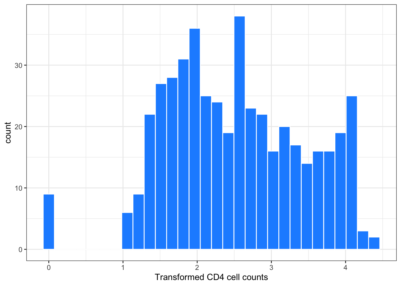
Figure 2: Histogram of transformed CD4 cell counts
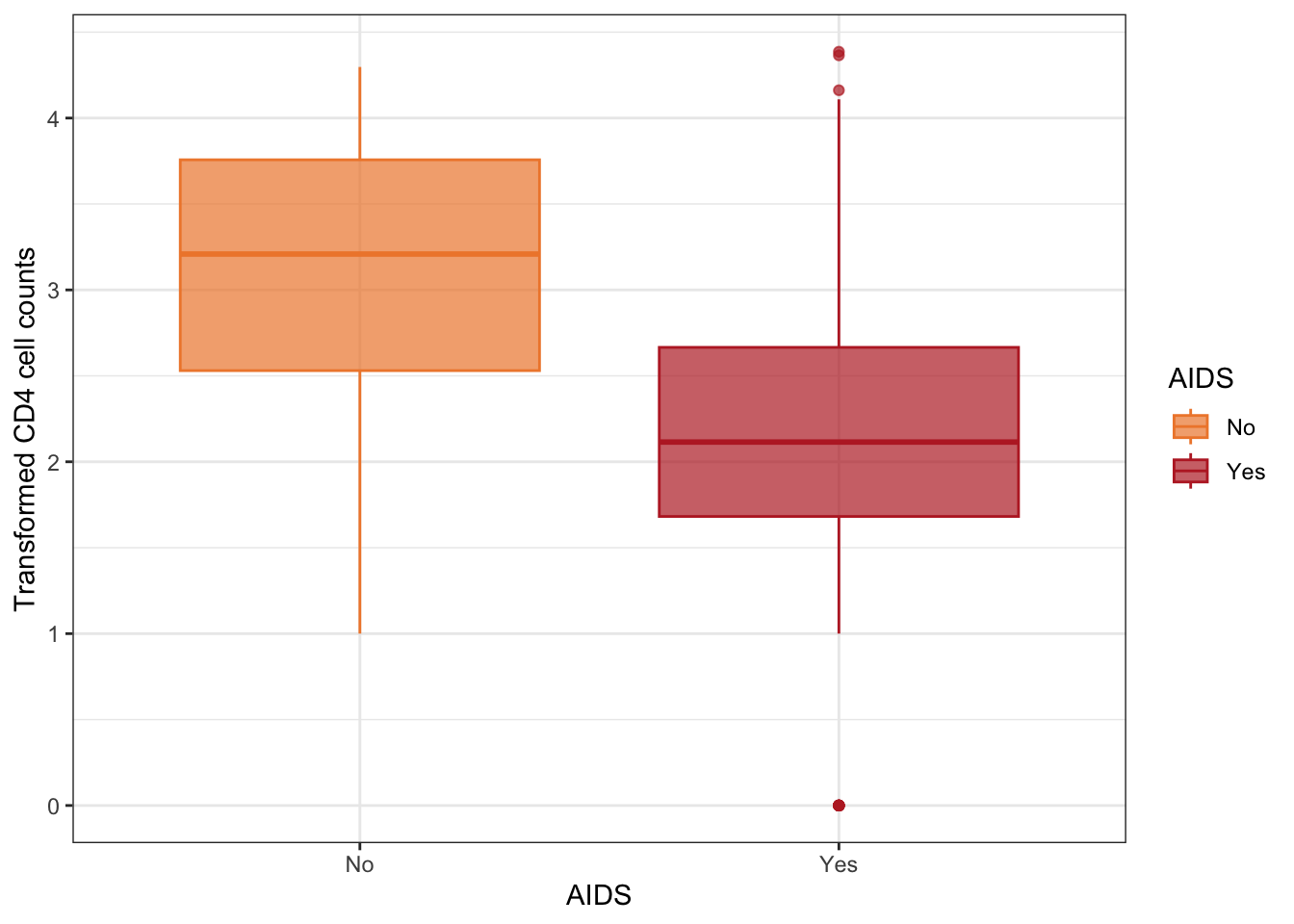
Figure 3: Boxplots of transformed CD4 cell counts according to AIDS status
Estimation
There are 3 unknown parameters in our model :
- \(\beta_0\)
- \(\beta_1\)
- \(\sigma\)
We will use the Maximum Likelihood Estimator for jointly estimating those 3 parameters.
First, let’s write the Gaussian likelihood. It is the product of the Gaussian likelihood contributions of each individual observation of y with individual mean \(\beta_0 +\beta_1 x_i\) and standard deviation \(\sigma\):
\[L(\beta_0, \beta_1, \sigma) =\prod_{i=1}^n \frac{1}{\sqrt{2\pi \sigma^2}} \exp\left(-\frac{\left(y_i - (\beta_0 +\beta_1 x_i)\right)^2}{2\sigma^2} \right)\]
We can transform this product as a sum when computing the log-likelihood \(\mathcal{L}(\beta_0, \beta1, \sigma)\): \[\mathcal{L} = -\frac{1}{2}\log(2\pi\sigma^2) - \sum_{i=1}^n\frac{\left(y_i - (\beta_0 +\beta_1 x_i)\right)^2}{2\sigma^2}\]
🫵 Practicals: your turn on
Make a function that takes
y,x,beta0,beta1, andsigmaas arguments and returns the corresponding likelihood contribution.#fill in the ... lik_contrib <- function(y, x, beta0, beta1, sigma){ l <- ... return(l) }Compute the likelihood observation of the first observation with
beta0=3,beta1=-5, andsigma=0.1. Compare it withbeta0=2,beta1=-7,sigma=0.2. Can you notice the problem ?lik_contrib(y=goldman1996$CD4t[1], x=goldman1996$AIDS[1], beta0=3, beta1=-5, sigma=0.1) lik_contrib(y=goldman1996$CD4t[1], x=goldman1996$AIDS[1], beta0=2, beta1=-7, sigma=0.2)Add a
logargument to youlik_contrib()function, which is set toTRUEby default and then computes the log-likelihood contribution (if set toFALSE, then the same computation as above is executed instead).#fill in the ... lik_contrib <- function(y, x, beta0, beta1, sigma, log=TRUE){ if(log) { contrib <- ... } else { contrib <- ... } return(...) }Use a
for-loop to compute the summed log-likelihood over all 467 observations.#fill in the ... n <- ... loglikelihood <- ... for (...){ ...[i] <- ... }sum(loglikelihood)Turn this loop into a function that takes a vector
paramof length 3 (c(beta0, beta1, sigma)) as its first argument, and theny(the outcome observation vector) andx(the covariate observation vector) as additional arguments.#fill in the ... loglik <- function(param, y, x){ b0 <- param[1] b1 <- param[2] s <- param[3] ... ... ... ... ... return(...) }Use the
optim()function to estimate the MLE for the 3 parameters.
Do not forget to set thecontrolargument equal tolist("fnscale"=-1)to ensuure that maximization is performed (instead of the default minimization).
Compare to the average values in the sample and to thelm()output.opt_res <- optim(par=c(0, 0, 0.1), fn = loglik, y=goldman1996$CD4t, x=goldman1996$AIDS, control=list("fnscale"=-1))beta0_MLE <- opt_res$par[1] beta0_MLE mean(goldman1996$CD4t[goldman1996$AIDS == 0]) beta1_MLE <- opt_res$par[2] beta1_MLE mean(goldman1996$CD4t[goldman1996$AIDS == 1]) - mean(goldman1996$CD4t[goldman1996$AIDS == 0]) sigma_MLE <- opt_res$par[3] sigma_MLE lm_res <- lm(CD4t~AIDS, data = goldman1996) sd(lm_res$residuals) summary(lm_res)
Below, two interactive graphics display respectively the likelihood and the log-likelihood surface around the MLE.