Exercise 1: Eliciting an expert prior

In the context of the historical example, we want to elicitate a prior distribution from expert knowledge.

Now, let’s imagine we have 2 expert demographers, each giving their expert opinion about the value they think plausible for $\theta$ (the probability of a birth being a girl rather than a boy).

We asks each of them to give values for which the probability of $\theta$ being lower would be respectively 10%, 25%, 50%, 75%, and 90%. First expert says: $$P(\theta <0.2)=10\mathrm{\%},P(\theta <0.4)=25\mathrm{\%},P(\theta <0.5)=50\mathrm{\%},P(\theta <0.6)=75\mathrm{\%},\text{and }P(\theta <0.8)=90\mathrm{\%}$$ while the second expert says: $$P(\theta <0.5)=10\mathrm{\%},P(\theta <0.6)=25\mathrm{\%},P(\theta <0.7)=50\mathrm{\%},P(\theta <0.8)=75\mathrm{\%},\text{and }P(\theta <0.9)=90\mathrm{\%}$$

0. First, let’s load the SHELF R package:

   library(SHELF)

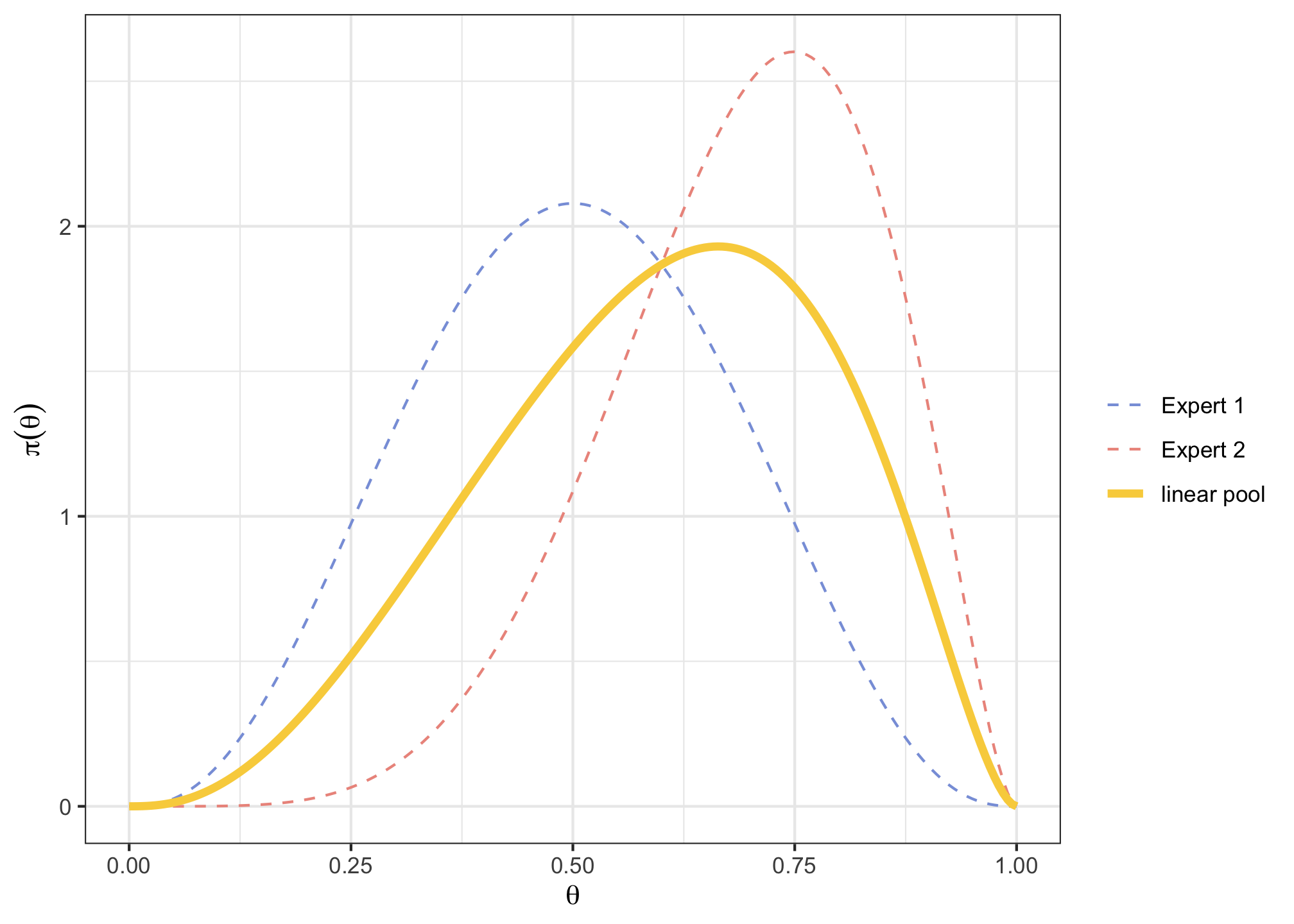
1. Using the fitdist() function from the SHELF package, estimate the parameter form the Beta distribution that best fit each of those elicitations (Protip: have a look at the package intro vignette here).

   v <- cbind(c(0.2, 0.4, 0.5, 0.6, 0.8),
              c(0.5, 0.6, 0.7, 0.8, 0.9)
   )
   p <- c(0.1, 0.25, 0.5, 0.75, 0.9)
   
   expertPriors <- fitdist(vals = v, probs = p, lower = 0, upper = 1,
                           expertnames=c("Expert 1", "Expert 2"))

   expertPriors$Beta

   ##            shape1   shape2
   ## Expert 1 3.634819 3.634835
   ## Expert 2 6.047483 2.692690

2. Plot those two Beta prior distributions, along with the “linear pooling” of their 2 curves using the plotfit() function from the SHELF package (Protip: use the lp = TRUE argument).

   expertPlot <- plotfit(expertPriors, d = "beta", lp = TRUE, xl = 0, xu = 1, 
                         xlab = expression(theta), ylab = expression(pi(theta)), 
                         returnPlot = TRUE)

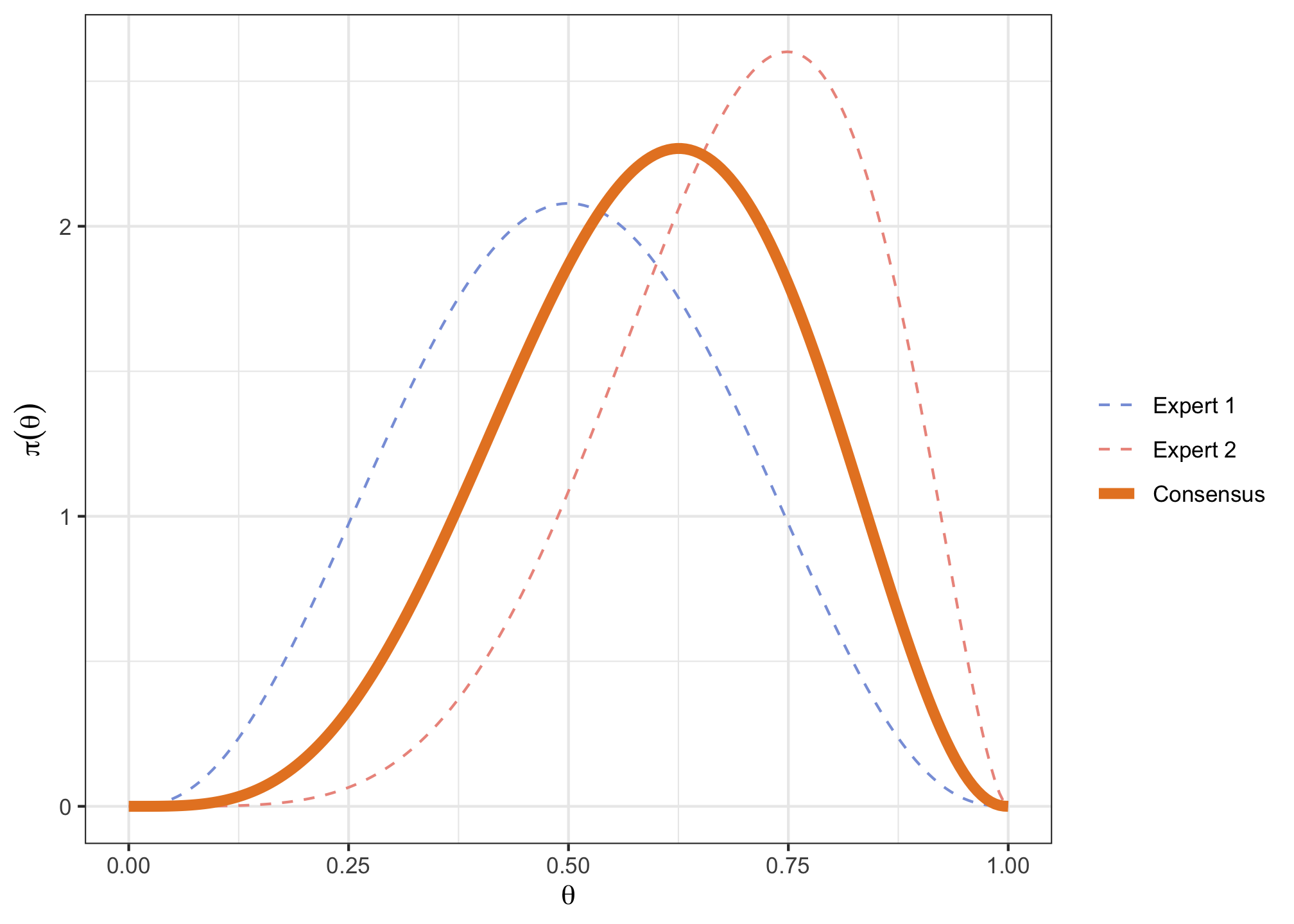
3. Derive a consensus Beta prior, by averaging each of both expert quantiles, and plot it.

   v <- cbind(c(0.2, 0.4, 0.5, 0.6, 0.8),
              c(0.5, 0.6, 0.7, 0.8, 0.9),
              c(0.35, 0.5, 0.6, 0.7, 0.85))
   p <- c(0.1, 0.25, 0.5, 0.75, 0.9)
   consensusPrior <- fitdist(vals = v, probs = p, lower = 0, upper = 1, 
                             expertnames=c("Expert 1", "Expert 2", "Consensus"))

   consensusPrior$Beta

   ##             shape1   shape2
   ## Expert 1  3.634819 3.634835
   ## Expert 2  6.047483 2.692690
   ## Consensus 4.822237 3.288318

   consensusPlot <- plotfit(consensusPrior, d = "beta", xl = 0, xu = 1, 
                            xlab = expression(theta), ylab = expression(pi(theta)), 
                            returnPlot = TRUE)