Exercise 2: Monte-Carlo

The Law of Large Numbers and Monte-Carlo Estimation.

1. Write a function which generates a sample of \(10\) observations \(iid\) from a Gaussian distribution (with mean \(m=2\) and standard deviation \(s=3\), i.e. a variance of \(9\)) and that returns the variance estimate over this sample (using the var() function).

   var_est <- function(n = 10) {
       s <- rnorm(n, mean = 2, sd = 3)
       return(var(s))
   }

2. Use the the Monte-Carlo method to estimate the variance of the distribution generating this sample, by using multiple realizations (e.g. 5) of the standard-deviation estimate implemented above. Do it again with 1,000 realizations, thus illustrating the law of large number convergence.

   # Monte-Carlo method
   nMC <- 5  # Monte Carlo sample size
   varMC <- numeric(nMC)
   for (i in 1:nMC) {
       varMC[i] <- var_est(n = 10)
   }
   mean(varMC)  # LLN estimate 
   
   nMC <- 1000  # Monte Carlo sample size
   for (i in 1:nMC) {
       varMC[i] <- var_est(n = 10)
   }
   mean(varMC)  # LLN estimate

Let’s now program a Monte-Carlo estimate of \(\pi\approx 3,1416\)

1. Program a function roulette_coord which has only one argument ngrid (representing the number of different outcomes possible on the roulette used) whose default is 35, generating the two coordinates of a point (between \(0\) and \(35\)) as a vector. Use the R function sample (whhose help page is accessible through the command ?sample). The function will return the vector of the 2 coordinates x and y generated this way.

   roulette_coord <- function(ngrid = 35) {
       x <- sample(x = 0:ngrid, size = 1)
       y <- sample(x = 0:ngrid, size = 1)
       return(c(x, y))
   }

2. Thanks to the formula to compute the distance bewteen 2 points: \(d = \sqrt{(x_1 - x_2)^2 + (y_1 - y_2)^2}\), program a function computing the distance to the origin (here has coordinates \((\frac{ngrid}{2}, \frac{ngrid}{2})\)) that checks if the computed distance is less than the unit disk radius (\(R = \frac{ngrid}{2}\)). This function, called for instance inside_disk_fun(), will have 2 arguments: the vector p containing the coordinates of the points on the one hand, and the integer ngrid on the other hand. It will return a boolean value (TRUEor FALSE) indicating the point is inside the disk.

   inside_disk_fun <- function(p, ngrid = 35) {
       d <- sqrt((p[1] - ngrid/2)^2 + (p[2] - ngrid/2)^2)
       return(d <= ngrid/2)
   }

3. The surface ratio between the disk (radius \(\frac{ngrid}{2}\)) and the square (side length \(ngrid\)) is equal to \(\frac{\pi}{4}\). This means that the probability of sampling a point inside the disk rather than outside is \(\frac{\pi}{4}\). Using this result, a Monte Carlo estimate of \(\pi\) can be implemented by computing the average number of time sampled points fall inside the disk multiplied by 4. Program such a function with their only input being a boolean vector of size \(n\) (the number of sampled points), which is TRUE if the point is indeed inside the disk and FALSE otherwise.

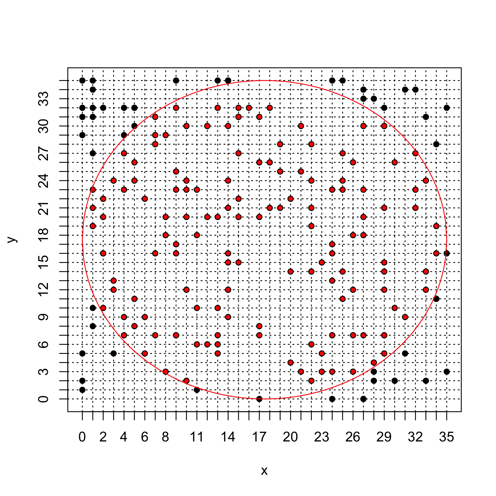
4. Using the code below, generate 200 points and plot the data generated. What is the corresponding Monte Carlo estimate of \(\pi\) ? Change npoints and comment. How could the estimation be improved (ProTip: try ngrid <- 1000 and npoints <- 5000) ?

   # Grid size (resolution)
   ngrid <- 35
   
   # Monte Carlo sample size
   npoints <- 200
   
   # Points generation
   pp <- matrix(NA, ncol = 2, nrow = npoints)
   for (i in 1:nrow(pp)) {
       pp[i, ] <- roulette_coord(ngrid)
   }
   
   # Estimate pi
   in_disk <- apply(X = pp, MARGIN = 1, FUN = inside_disk_fun, ngrid = ngrid)
   piMC(in_disk)
   
   # Plot first we initialise an empty plot with the right size using argument
   plot(x = pp[, 1], y = pp[, 2], xlim = c(0, ngrid), ylim = c(0, ngrid), axes = 0,
       xlab = "x", ylab = "y", type = "n")
   ## we tick the x and then y axes from 1 to ngrid
   axis(1, at = c(0:ngrid))
   axis(2, at = c(0:ngrid))
   ## we add a square around the plot
   box()
   ## we plot the grid (using dotted lines thanks to the argument `lty = 3`) onto
   ## which the points are sample
   for (i in 0:ngrid) {
       abline(h = i, lty = 3)
       abline(v = i, lty = 3)
   }
   ## we add the sampled points
   lines(x = pp[, 1], y = pp[, 2], xlim = c(0, ngrid), ylim = c(0, ngrid), xlab = "x",
       ylab = "y", type = "p", pch = 16)
   ## we add the circle display
   x.circle <- seq(0, ngrid, by = 0.1)
   y.circle <- sqrt((ngrid/2)^2 - (x.circle - ngrid/2)^2)
   lines(x.circle, y = y.circle + ngrid/2, col = "red")
   lines(x.circle, y = -y.circle + ngrid/2, col = "red")
   ## finally we color in red the points sampled inside the disk
   lines(x = pp[in_disk, 1], y = pp[in_disk, 2], xlim = c(0, ngrid), ylim = c(0, ngrid),
       xlab = "x", ylab = "y", type = "p", pch = 16, col = "red", cex = 0.7)