Exercise 3: Inverse transform sampling

Program a sampling algorithm to sample from the exponential distribution with parameter \(\lambda\) thanks to the inverse transform function (starting from the R function runif).
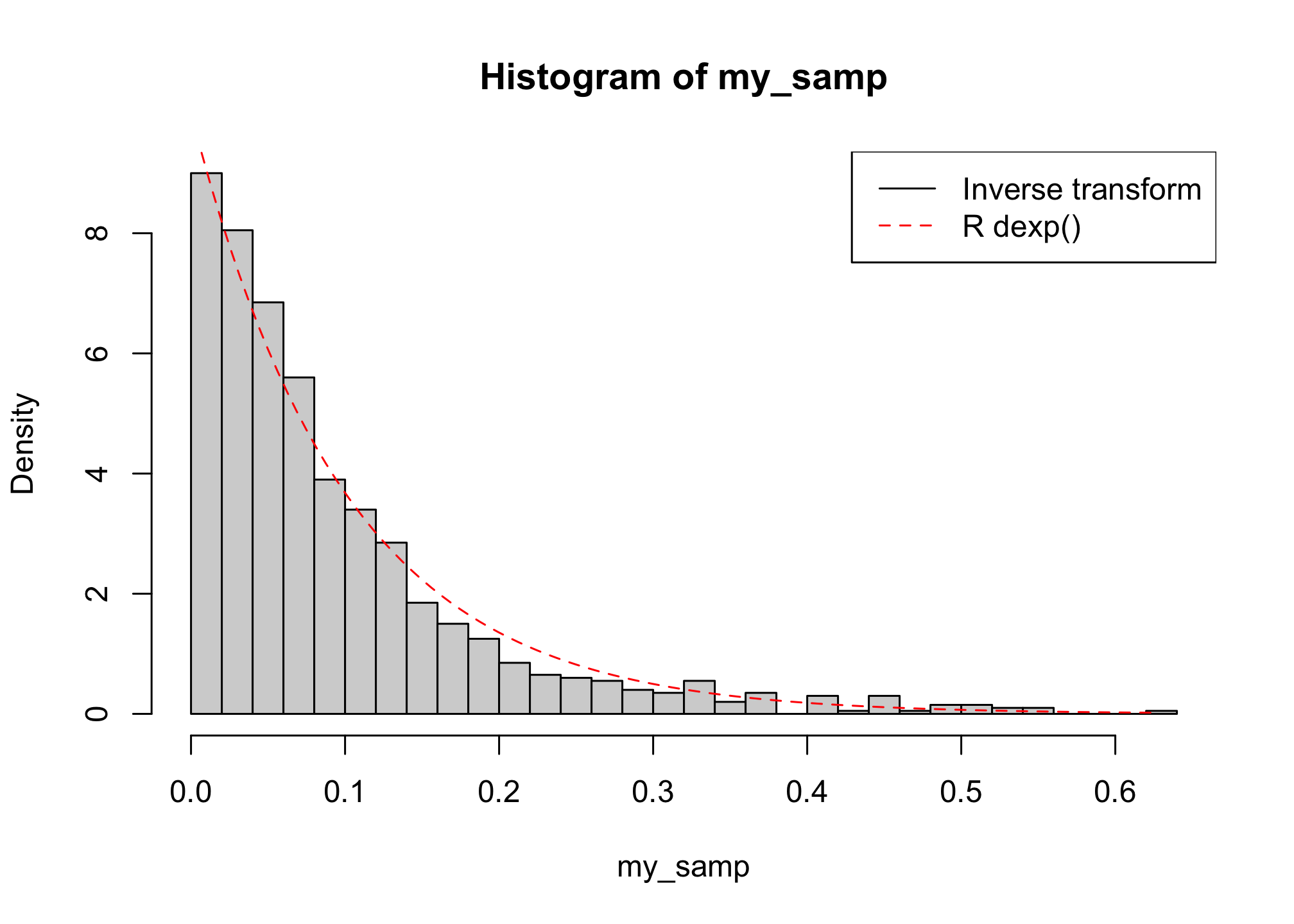
Compare the distribution of your sample to the theoretical target distribution (thanks to the built-in R function dexp).
Try out several values for the \(\lambda\) parameter of the exponential distribution (e.g. 1, 10, 0.78, …) to check that the algorithm is indeed working.

generate_exp <- function(n, lambda) {
    u <- ...
    x <- ...
    return(x)
}
my_samp <- generate_exp(n = 100, lambda = 10)
hist(my_samp, probability = TRUE, n = 25)
curve(dexp(x, rate = 10), from = 0, to = max(my_samp), col = "red", lty = 2, add = TRUE)
legend("topright", c("Inverse transform", "R dexp()"), col = c("black", "red"), lty = c(1,
    2))