Exercise 4: Metropolis-Hastings algorithm(s) for the historical application (Beta-Bernoulli model)

Using the historical example, program an independent Metropolis-Hastings algorithm to estimate the posterior distribution of parameter $\theta$ (i.e. the probability of having a girl for a birth). The prior distribution on $\theta$ will be used as the instrumental proposal, and we will start by using a uniform prior on $\theta$. We will consider the $493,472$ births observed in Paris between 1745 and 1770, of which $241,945$ were girls.

1. Program a function that computes the numerator of the posterior density, which can be written $p(\theta |n,S)\propto {\theta }^S(1-\theta {)}^{n-S}$ with $S=241945$ and $n=493472$ (plan for a boolean argument that will allow to return — or not — the logarithm of the posterior instead).

   post_num_hist <- function(theta, log = FALSE) {
   
       n <- 493472  # the data
       S <- 241945  # the data
   
       if (log) {
           num <- S * log(theta) + (n - S) * log(1 - theta)  # the **log** numerator of the posterior
       } else {
           num <- theta^S * (1 - theta)^(n - S)  # the numerator of the posterior
       }
       return(num)  # the output of the function
   }
   
   post_num_hist(0.2, log = TRUE)

   ## [1] -445522.1

   post_num_hist(0.6, log = TRUE)

   ## [1] -354063.6

2. Program the corresponding Metropolis-Hastings algorithm, returning a vector of size $n$ sampled according to the posterior distribution. Also, have the algorithm return the vector of acceptance probabilities $\alpha$. What happens if this acceptance probability is NOT computed on the $log$ scale ?

   myMH <- function(niter, post_num) {
   
       x_save <- numeric(length = niter)  #create a vector of 0s 
       # of length niter to store the sampled values
   
       alpha <- numeric(length = niter)  #create a vector of 0s 
       # of length niter to store the acceptance probabilities
   
       # initialise x0
       x <- runif(n = 1, min = 0, max = 1)
   
       # acceptance-rejection loop
       for (t in 1:niter) {
           # sample y from the proposal (here uniform prior)
           y <- runif(n = 1, min = 0, max = 1)
           # compute the acceptance-rejection probability
           alpha[t] <- min(1, exp(post_num(y, log = TRUE) - post_num(x, log = TRUE)))
           # accept or reject
           u <- runif(1)
           if (u <= alpha[t]) {
               x_save[t] <- y
           } else {
               x_save[t] <- x
           }
   
           # update the current value
           x <- x_save[t]
       }
       return(list(theta = x_save, alpha = alpha))
   }

3. Compare the posterior density obtained with this Metropolis-Hastings algorithm over 2000 iterations to the theoretical one (the theoretical density can be obtained with the R function dbeta(x, 241945 + 1, 251527 + 1) and represented with the R function curve(..., from = 0, to = 1, n = 10000)). Mindfully discard the first 500 iterations of your Metropolis-Hastings algorithm in order to reach the Markov chain convergence before constructing your Monte Carlo sample. Comment those results, especially in light of the acceptance probabilities computed throughout the algorithm, as well as the different sampled values for $\theta$.

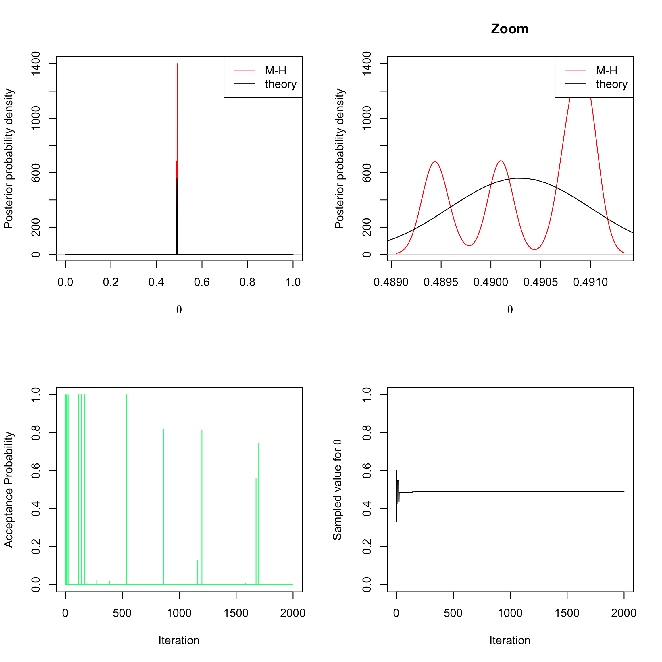
4. Now imagine we only observe $100$ births, among which $49$ girls, and use a $\text{Beta}(\alpha =3,\beta =3)$ distribution as prior. Program the corresponding M-H algorithm and study the new results (one can do $10,000$ iterations of this new M-H algorithm for instance, again mindfully discarding the first 500 iterations).

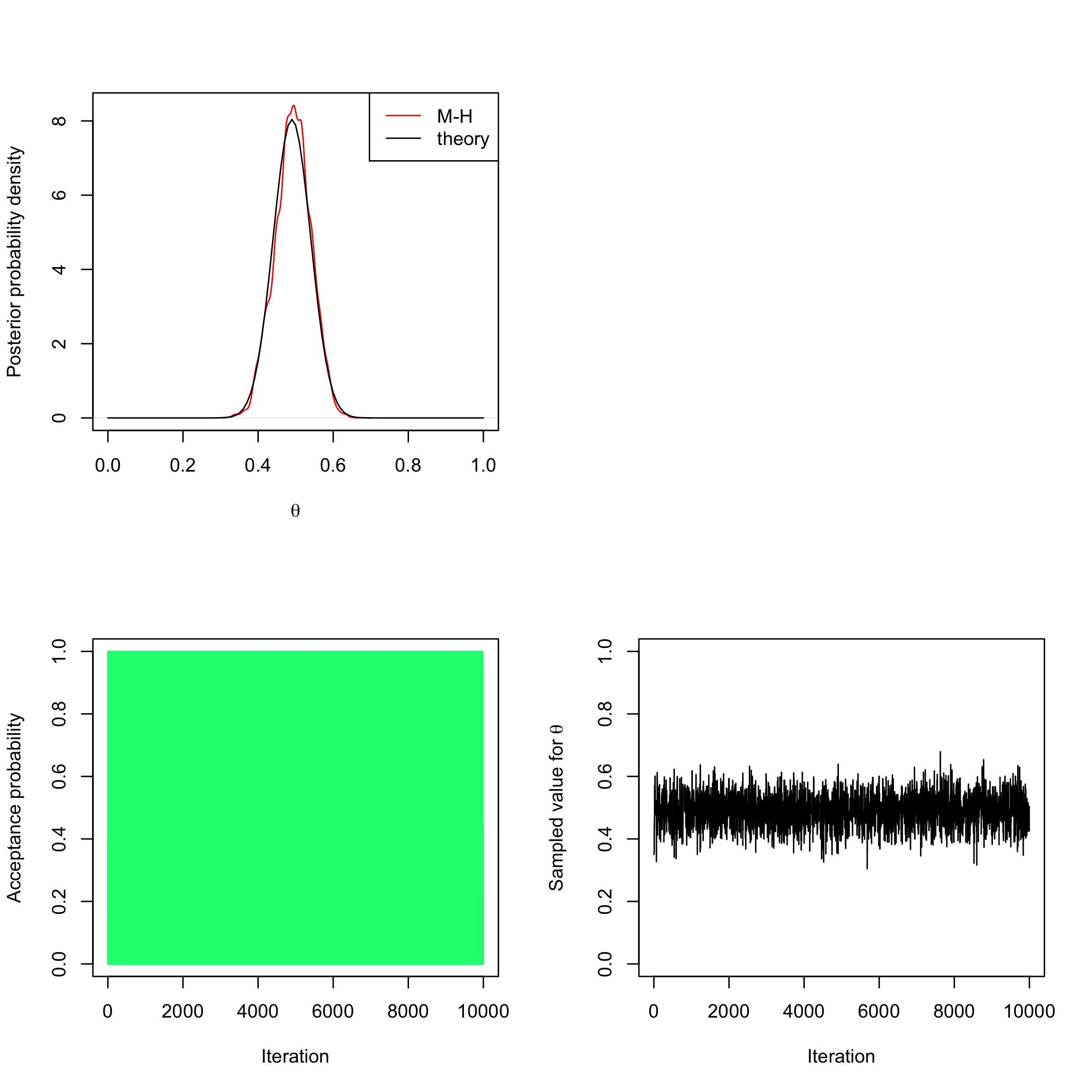
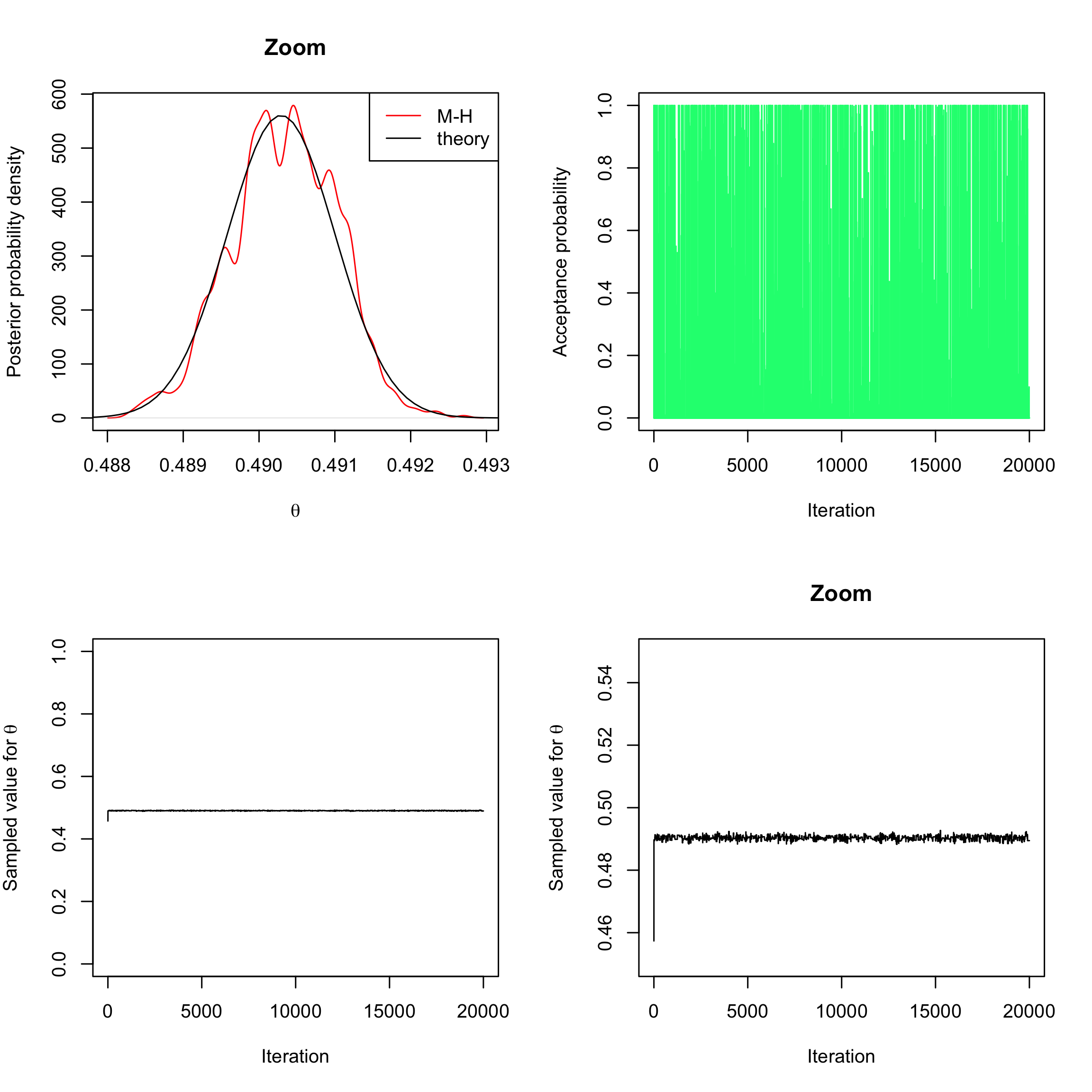
5. Using the data from the historical example and with a $\text{Beta}(\alpha =3,\beta =3)$ prior, program a random-walk Metropolis-Hastings algorithm (with a Gaussian random step of sd=0.02 for instance). This means that the proposal is going to change, and is now going to depend on the previous value.
   Once again, study the results obtained this way (one can change the width of the random step).