Exercise 5: Introduction to BUGS & JAGS

The BUGS project (Bayesian inference Using Gibbs Sampling) was initiated in 1989 by the MRC (Medical Research Council) Biostatistical Unit at the University of Cambridge (United-Kingdom) to develop a flexible and user-friendly software for Bayesian analysis of complex models through MCMC algorithms. Its most famous and original implementation is WinBUGS, a clicking software available under Windows. OpenBUGS is an alternative implementation of WinBUGS running on either Windows, Mac OS ou Linux. JAGS (Just another Gibbs Sampler) is a different and newer implementation that also relies on the BUGS language. Finally, the STAN software must also be mentionned, recently developed et the Columbia Univeristy, ressemble BUGS through its interface, but relies on innovative MCMC approaches, such as Hamiltonian Monte Carlo, or variational Bayes approaches. A very useful resource is the JAGS user manual.

To familiarise yourself with JAGS (and its R interface through the package rjags), we will look here at the posterior estimation of the mean and variance of observed data that we will model with a Gaussian distribution.

Start by loading the R package rjags.
```
library(rjags)
```

A BUGS model has 3 components:

the model: specified in an external text file (.txt) according to a specific BUGS syntax
the data: a list containing each observation under a name matching the one used in the model specification
the initial values: (optional) a list containing the initial values for the various parameters to be estimated

Sample $N = 50$ observations from a Gaussian distribution with mean $m = 2$ and standard deviation $s = 3$ using the R function rnorm and store it into an object called obs.
```
N <- 50  # the number of observations
obs <- rnorm(n = N, mean = 2, sd = 3)  # the (fake) observed data
```

Read the help of the rjags package, then save a text file (.txt) the following code defining the BUGS model:

# Model
model{

  # Likelihood
  for (i in 1:N){ 
    obs[i]~dnorm(mu,tau)
  }

  # Prior
  mu~dnorm(0,0.0001) # proper but very flat (so weakly informative)
  tau~dgamma(0.0001,0.0001) # proper, and weakly informative (conjugate for Gaussian)

  # Variables of interest
  sigma <- pow(tau, -0.5)
}

Each model specification file must start with the instruction model{ indicating JAGS is about to receive a model specification. Then the model must be set up, usually by cycling along the data with a for loop. Here, we want to declare N observations, and each of them obs[i] follows a Gaussian distribution (characterized with the command dnorm) of mean mu and precision tau.

⚠️ In BUGS, the Gaussian distribution is parameterized by its precision, which is simply the inverse of the variance ( $τ = 1 / σ^{2}$ ). Then, one needs to define the prior distribution for each parameter -– here both mu and tau. For mu, we use a Gaussian prior with mean $0$ and precision $10^{- 4}$ (thus variance $10, 000$ : this corresponds to a weakly informative prior quite spread out given the scale of our data. For tau we use the conjugate prior for precision in a Gaussian model, namely the Gamma distribution (with very small parameters, here again to remain the least informative possible). Finally, we give a deterministic definition of the additional parameters of interest, here the standard deviation sigma.

NB: ~ indicates probabilistic distribution definition of a random variable, while <- indicates a deterministic calculus definition.

With the R function jags.model(), create a jags object R.

myfirstjags <- jags.model("normalBUGSmodel.txt", data = list(obs = obs, N = length(obs)))

## Compiling model graph
##    Resolving undeclared variables
##    Allocating nodes
## Graph information:
##    Observed stochastic nodes: 50
##    Unobserved stochastic nodes: 2
##    Total graph size: 58
## 
## Initializing model

With the R function coda.samples(), generate a sample of size $2, 000$ from the posterior distributions for the mean and standard deviation parameters.
```
res <- coda.samples(model = myfirstjags, variable.names = c("mu", "sigma"), n.iter = 2000)
```

Study the output of the coda.samples() R function, and compute both the posterior mean and median estimates for mu and sigma. Give a credibility interval at 95% for both.

plot(res)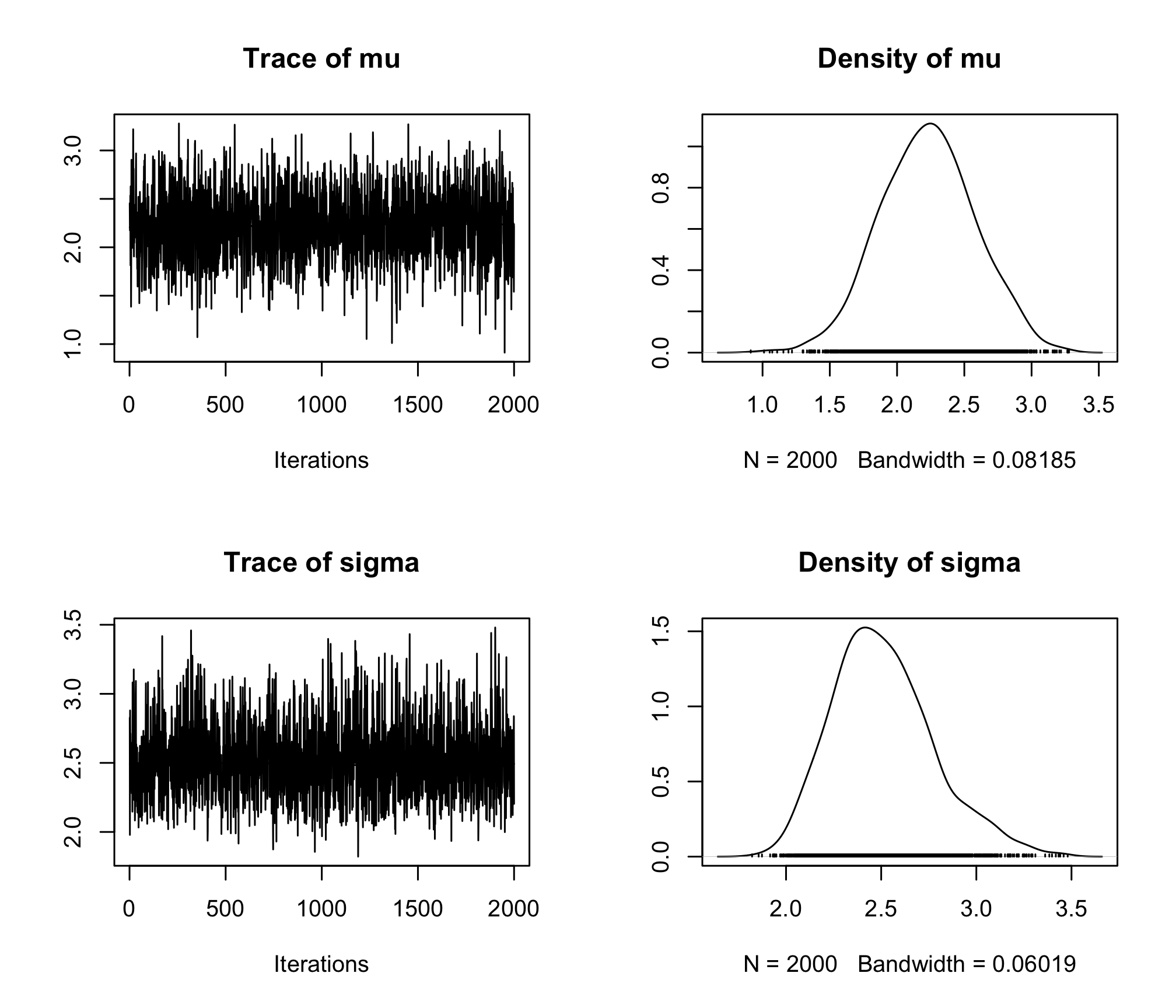

res_sum <- summary(res)
res_sum

## 
## Iterations = 1:2000
## Thinning interval = 1 
## Number of chains = 1 
## Sample size per chain = 2000 
## 
## 1. Empirical mean and standard deviation for each variable,
##    plus standard error of the mean:
## 
##        Mean     SD Naive SE Time-series SE
## mu    2.228 0.3542 0.007921       0.007921
## sigma 2.512 0.2669 0.005968       0.006224
## 
## 2. Quantiles for each variable:
## 
##        2.5%   25%   50%   75% 97.5%
## mu    1.536 1.987 2.232 2.460 2.913
## sigma 2.069 2.324 2.484 2.672 3.108

res_sum$statistics["mu", "Mean"]

## [1] 2.228383

res_sum$statistics["sigma", "Mean"]

## [1] 2.511918

res_sum$quantiles["mu", "50%"]

## [1] 2.231571

res_sum$quantiles["sigma", "50%"]

## [1] 2.484006

res_sum$quantiles["mu", c(1, 5)]

##     2.5%    97.5% 
## 1.535557 2.913115

res_sum$quantiles["sigma", c(1, 5)]

##     2.5%    97.5% 
## 2.068717 3.107573

Load the coda R package. This package functions for convergence diagnostic and analysis of MCMC algorithm outputs.
```
library(coda)
```

To diagnose the convergence of an MCMC algorithm, it is necessary to generate different Markov chains, with different initial values. Recreate a new jags object in R and specify the use of 3 Markov chains with the argument n.chains, and initialize mu at $0, - 10, 100$ and tau at $1, 0.01, 0.1$ respectively with the argument inits (ProTip: use a list of list, one for each chain).

myjags2 <- jags.model("normalBUGSmodel.txt", data = list(obs = obs, N = N), n.chains = 3,
    inits = list(list(mu = 0, tau = 1), list(mu = -10, tau = 1/100), list(mu = 100,
        tau = 1/10)))

## Compiling model graph
##    Resolving undeclared variables
##    Allocating nodes
## Graph information:
##    Observed stochastic nodes: 50
##    Unobserved stochastic nodes: 2
##    Total graph size: 58
## 
## Initializing model

res2 <- coda.samples(model = myjags2, variable.names = c("mu", "sigma"), n.iter = 1000)
plot(res2)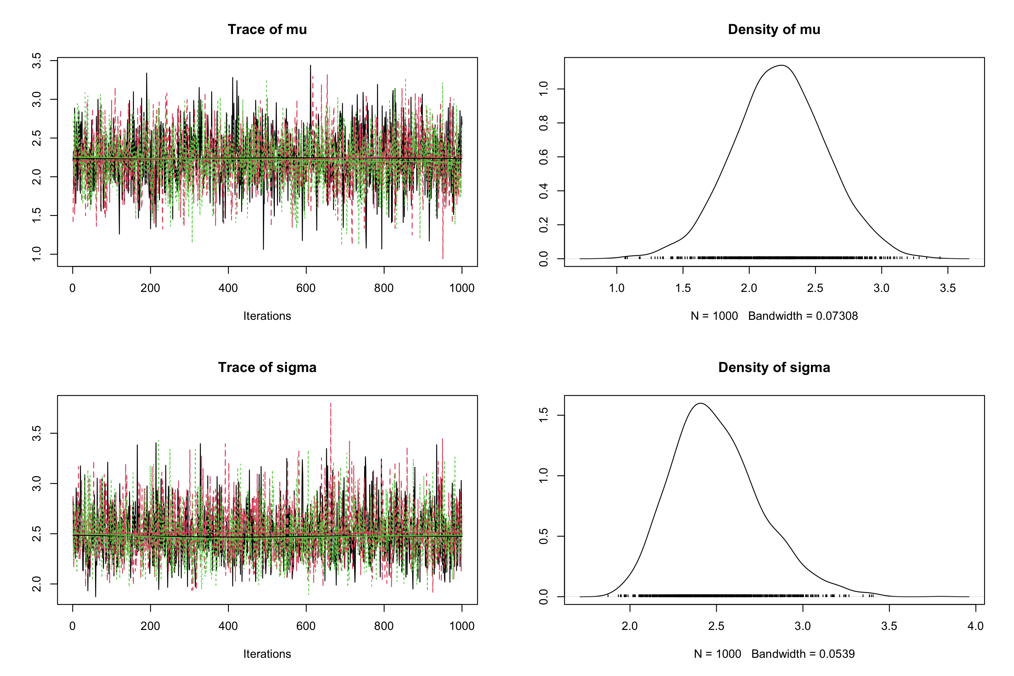

With the R function gelman.plot(), plot the Gelman-Rubin statistic.
```
gelman.plot(res2)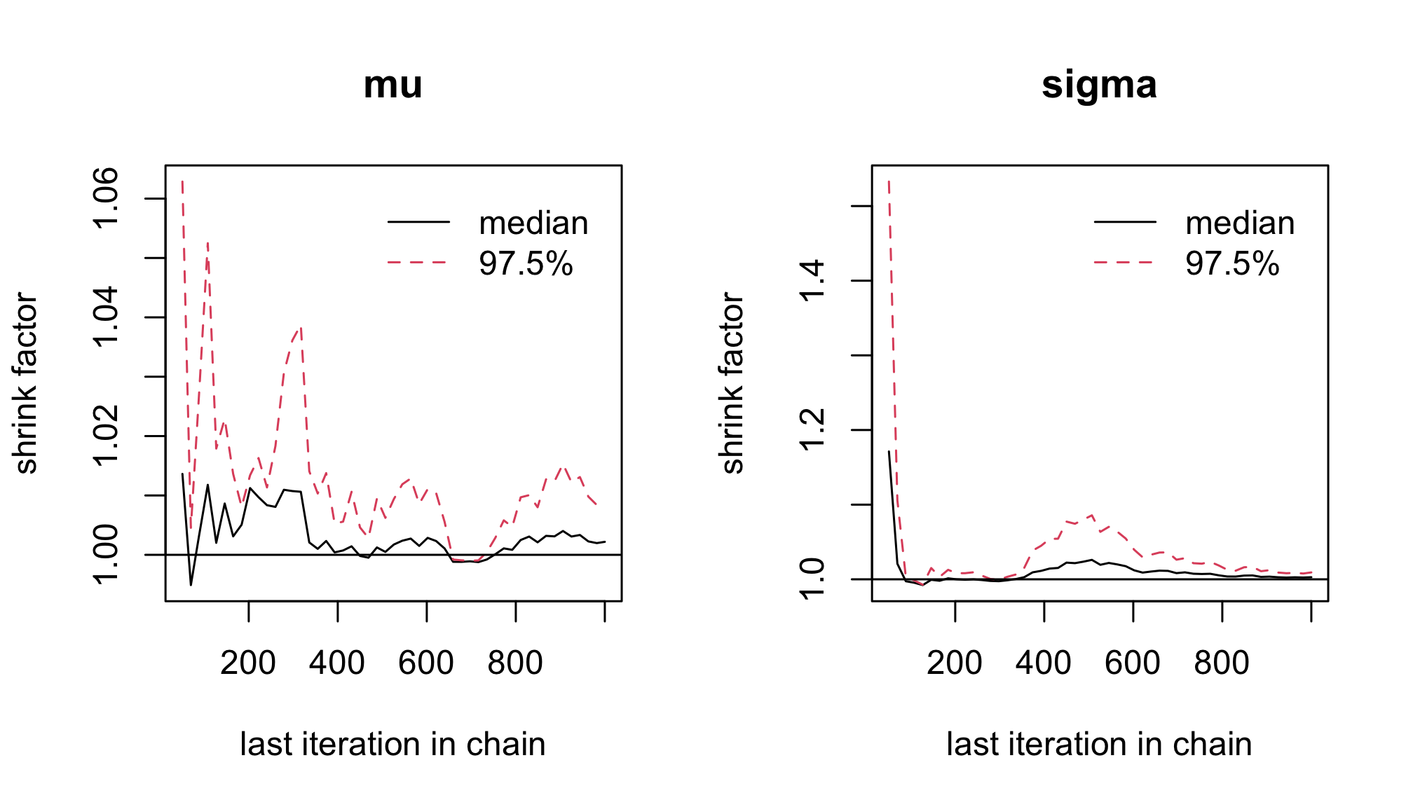
```
With the R functions autocorr.plot() and acfplot() evaluate the autocorrelation of the studied parameters.
```
acfplot(res2)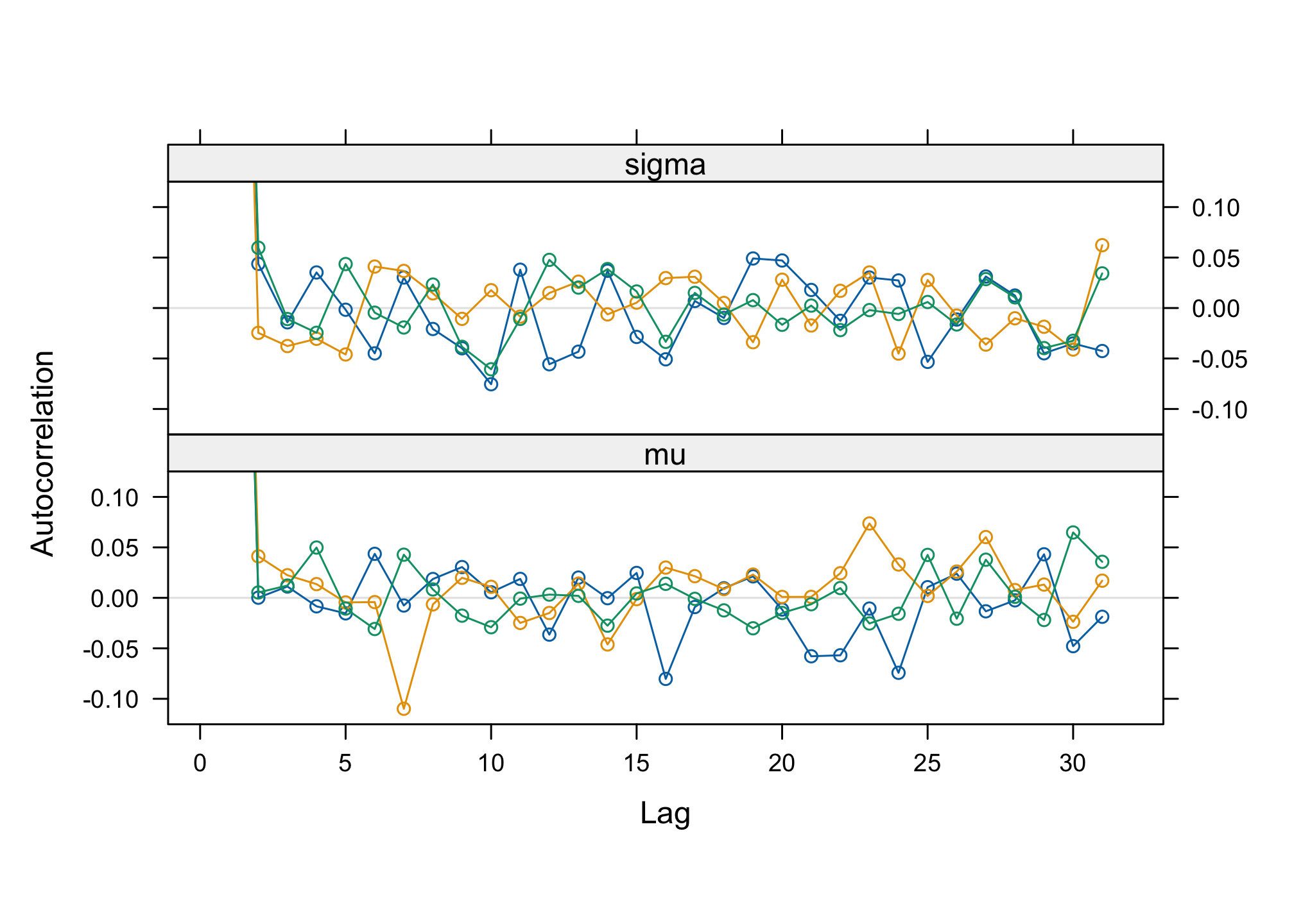
```
```
par(mfrow = c(3, 2))
autocorr.plot(res2, ask = FALSE, auto.layout = FALSE)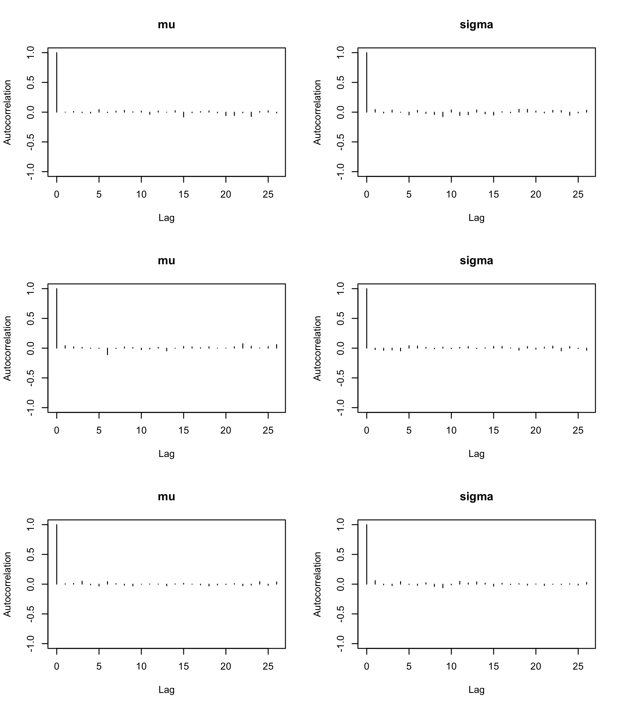
```
With the R function cumuplot() evaluate the running quantiles of the studied parameters. How can you interpret them ?
```
par(mfrow = c(3, 2))
cumuplot(res2, ask = FALSE, auto.layout = FALSE)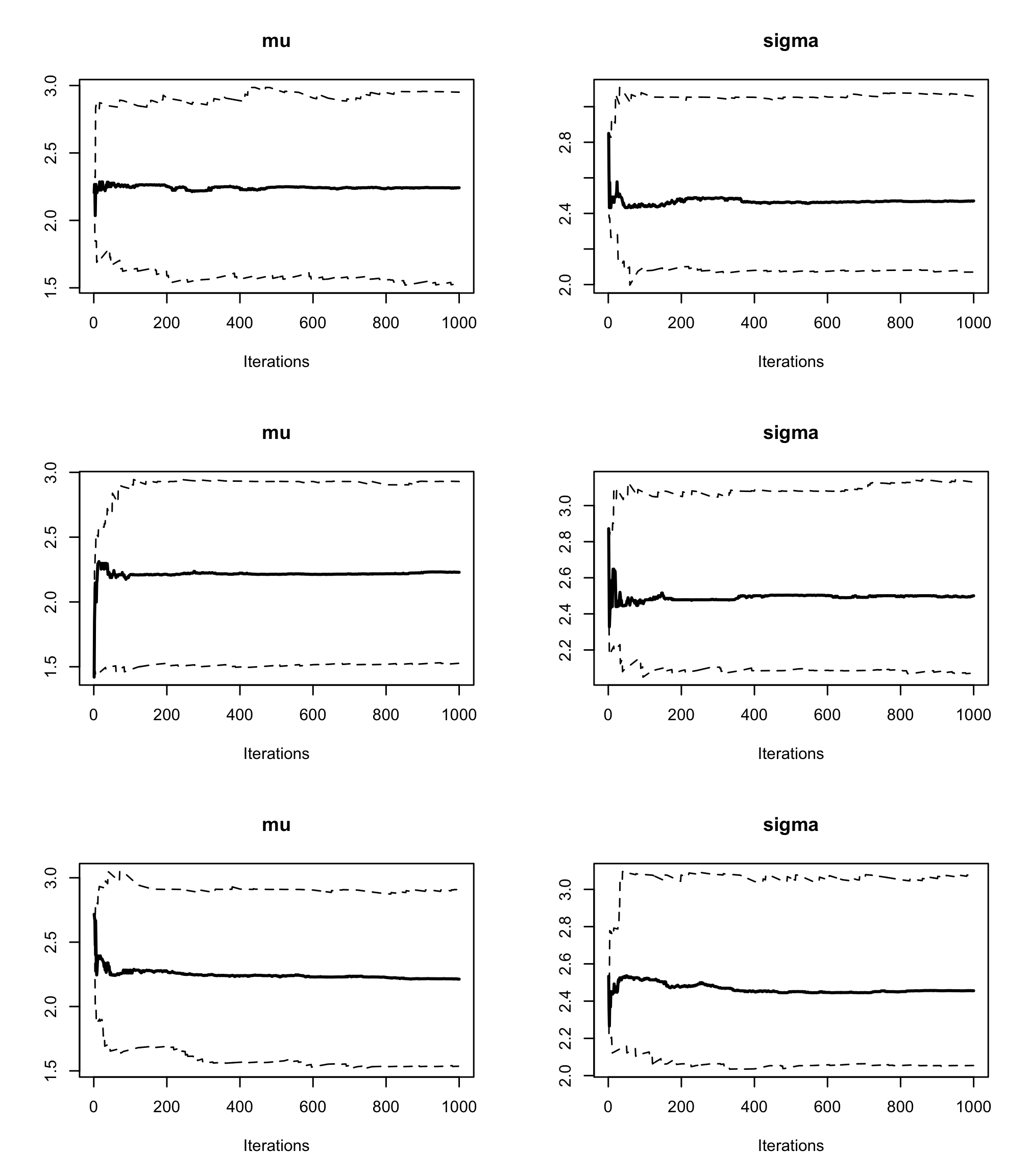
```
Each row of the above graph is a different chain. The cumulative quantiles are indeed stable after the first few iterations in all chains.

With the function hdi() from the R package HDInterval, provide highest densitity posterior credibility intervals at 95%, and compare them to those obtained with the $2.5$ % and $97.5$ % quantiles.

hdCI <- HDInterval::hdi(res2)
hdCI

##             mu    sigma
## lower 1.544911 2.015604
## upper 2.933025 3.018926
## attr(,"credMass")
## [1] 0.95

symCI <- summary(res2)$quantiles[, c(1, 5)]
symCI

##           2.5%    97.5%
## mu    1.532256 2.927862
## sigma 2.064821 3.085987

symCI[, 2] - symCI[, 1]

##       mu    sigma 
## 1.395606 1.021166

hdCI[2, ] - hdCI[1, ]

##       mu    sigma 
## 1.388114 1.003322

Last updated on October 30, 2025

Edit this page