Probability of Success exercises
Exercise 1: propose a sample size for the confirmatory trial
Requirements/assumptions:
- We would like to have a power of 90%
- We would like to control the false positive rate at a one-sided 2.5% level
- Make appropriate assumptions about:
- the expected difference \(\delta\) in mean CFB in MMD at week 12
- the standard deviation \(\sigma\) for the CFB in MMD at week 12
The sample size per arm is given by the following formula:
\[ n = \dfrac{2 \sigma^2 (Z_{1-\alpha} + Z_{1-\beta})^2}{\delta^2}\]
NB: remember that the power is \(1-\beta\), so \(\beta=10\%\).
If we use the quantities from the previous trial at week 4 as guesses for \(\delta = -2\) and \(\sigma = 6.5\), the necessary sample size per arm is estimated at 222.
The right choice for the standard deviation and expected effect size can be debated due to design differences between the proof of concept trial and the confirmatory trial. One could also consider powering the study for the minimum relevant effect from either a clinical or a business perspective.
# Assumptions:
delta <- -2
sigma <- 6.5
power <- 0.9
beta <- 1 - power
alpha <- 0.025
# Sample size computation
sample_size <- 2 * sigma^2 * (qnorm(1 - alpha) + qnorm(1 - beta))^2/delta^2
ceiling(sample_size)## [1] 222The right choice for the standard deviation and expected effect size can be debated due to design differences between the proof of concept trial and the confirmatory trial. One could also consider powering the study for the minimum relevant effect from either a clinical or a business perspective.
Exercise 2: calculate assurance for the confirmatory trial
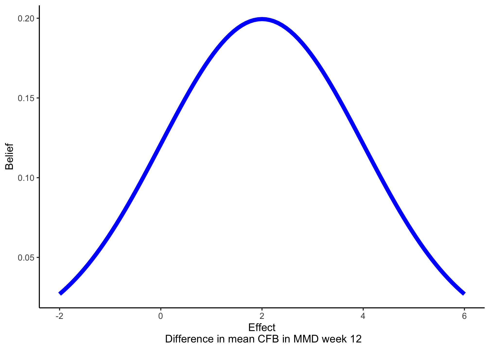
Use a normal distribution with mean 2 and standard deviation 2 as prior.
Create a plot with sample size (from 1 to 1000) on the x-axis and PoS on the y-axis. Include first one curve displaying power as a function of the sample size, and second one curve displaying assurance as a function of sample size.
Hint: first create two functions that return power and assurance as a function of sample size using formulas from slides #31 and #13 (if you need help, see last slide in this presentation).# Hint power_fun <- function(n, delta = 2, sigma = 6.5, alpha = 0.025) { # TODO from slide n°13 } assurance_fun <- function(n, mu_delta = 2, sigma_delta = 2, sigma = 6.5, alpha = 0.025) { # TODO from slide n°31 }# Coding tip: use the apply function to quickly obtain the value of a # function for a sequence of input values n <- seq(0,1000,1) results <- sapply(n, _yourfunction_, ...) #where you can use ... to # give further arguments # to _yourfunction_power_fun <- function(n, delta = 2, sigma = 6.5, alpha = 0.025) { pwr <- pnorm(qnorm(alpha) + (sqrt(n) * delta)/(sqrt(2) * sigma)) return(pwr) } assurance_fun <- function(n, mu_delta = 2, sigma_delta = 2, sigma = 6.5, alpha = 0.025) { tau <- sigma * sqrt(2/n) asrc <- pnorm((-qnorm(1 - alpha) * tau + mu_delta)/(sqrt(sigma_delta^2 + tau^2))) return(asrc) }# Ploting the results n <- seq(1, 1000, 1) power_res <- sapply(n, power_fun) assurance_res <- sapply(n, assurance_fun) plot(x = n, power_res, xlab = "Sample size per arm", ylab = "PoS", type = "l", col = "red3", ylim = c(0, 1), lwd = 1.5) lines(x = n, assurance_res, type = "l", col = "dodgerblue", ylim = c(0, 1), lty = "dashed", lwd = 1.5) legend("bottomright", legend = c("Power", "Assurance"), col = c("red3", "dodgerblue"), lty = c("solid", "dashed"), lwd = 1.5)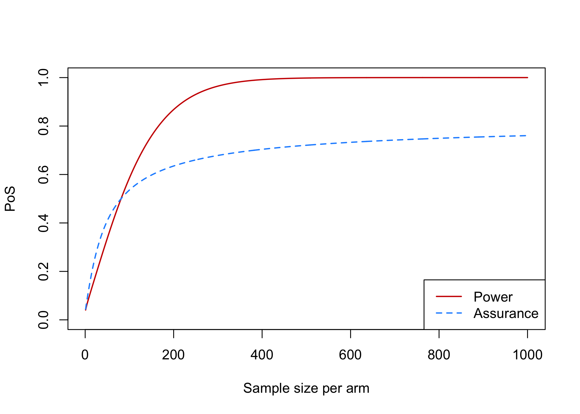
What is the assurance for the sample size you calculated in Exercise 1 ? Would you choose a different sample size based on assurance?
assurance_fun(n = 222)## [1] 0.6472213What is the upper bound for assurance for this example? What is the interpretation of this upper bound?
assurance_fun(n = 1000)
assurance_fun(n = 10^6)
assurance_fun(n = 10^10)
assurance_fun(n = 10^200)
## [1] 0.7604324 ## [1] 0.8391526 ## [1] 0.8413229 ## [1] 0.8413447The upper bound can be obtained by either inserting a very large sample size in your assurance function (approximation) or precisely by integrating the region under the prior where the effect is greater than 0.
n_log <- exp(seq(1,15,0.25))
power_res <- sapply(n_log, power_fun)
assurance_res <- sapply(n_log, assurance_fun)

library(ggplot2)
ggplot(cbind.data.frame(n_log, power_res, assurance_res), aes(x=n_log)) +
  geom_line(aes(y=power_res, linetype="Power", color="Power")) +
  geom_line(aes(y=assurance_res, linetype="Assurance", color="Assurance")) +
  scale_linetype_manual(name="", values=c("dashed", "solid")) +
  scale_color_manual(name="", values=c("dodgerblue", "red3")) +
  ylab("PoS") +
  xlab("Sample size per arm (log scale)") +
  ylim(c(0,1)) +
  theme_bw() +
  scale_x_log10() +
  annotation_logticks(sides = "b")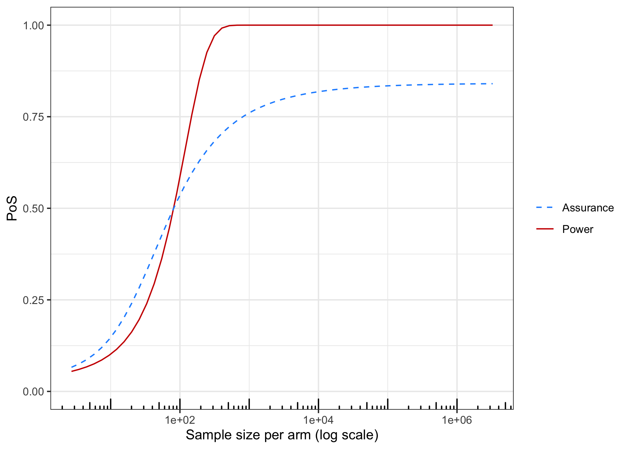
# theoretical upper bound: part of the prior for values below zero
1 - pnorm(0, mean = 2, sd = 2)
## [1] 0.8413447The minimum value that results in a significant p-value is \(1.21\)
min_sig <- 6.5 * sqrt(2/222) * qnorm(0.975)
min_sig
## [1] 1.209205
Exercise 3: adding a requirement on the minimum relevant effect to assurance
To the plot from Exercise 2, add a line for assurance where success is declared if the p-value is significant AND the effect estimate is at least \(1.5\).
Hint: modify the formula from slide #31For this version of assurance we declare success if \[\bar{y}_1 - \bar{y}_0 > z_{1-\alpha}\tau \quad \text{and} \quad \bar{y}_1 - \bar{y}_0 > 1.5\] The formula from Slide 31 can be modified as follows:
\[P\left[\bar{y}_1 - \bar{y}_0 > \max(z_{1-\alpha}\tau,1.5)\right] = \Phi\left(\frac{-\max(z_{1-\alpha}\tau,1.5) + \mu_{\delta}}{\sqrt{\sigma^2_{\delta}+\tau^2}}\right)\]assurance_fun_both <- function(n, mre = 1.5, mu_delta = 2, sigma_delta = 2, sigma = 6.5, alpha = 0.025) { tau <- sigma * sqrt(2/n) asrc <- pnorm((-max(qnorm(1 - alpha) * tau, mre) + mu_delta)/(sqrt(sigma_delta^2 + tau^2))) return(asrc) }n <- seq(1, 1000, 1) power_res <- sapply(n, power_fun) assurance_res <- sapply(n, assurance_fun) assurance_res_both <- sapply(n, assurance_fun_both) plot(x = n, power_res, xlab = "Sample size per arm", ylab = "PoS", type = "l", col = "red3", ylim = c(0, 1), lwd = 1.5) lines(x = n, assurance_res, type = "l", col = "dodgerblue", ylim = c(0, 1), lty = "dashed", lwd = 1.5) lines(x = n, assurance_res_both, type = "l", col = "orange", ylim = c(0, 1), lty = "dotted", lwd = 1.5) legend("bottomright", legend = c("Power", "Assurance - pval", "Assurance - pval & effect"), col = c("red3", "dodgerblue", "orange"), lty = c("solid", "dashed", "dotted"), lwd = 1.5)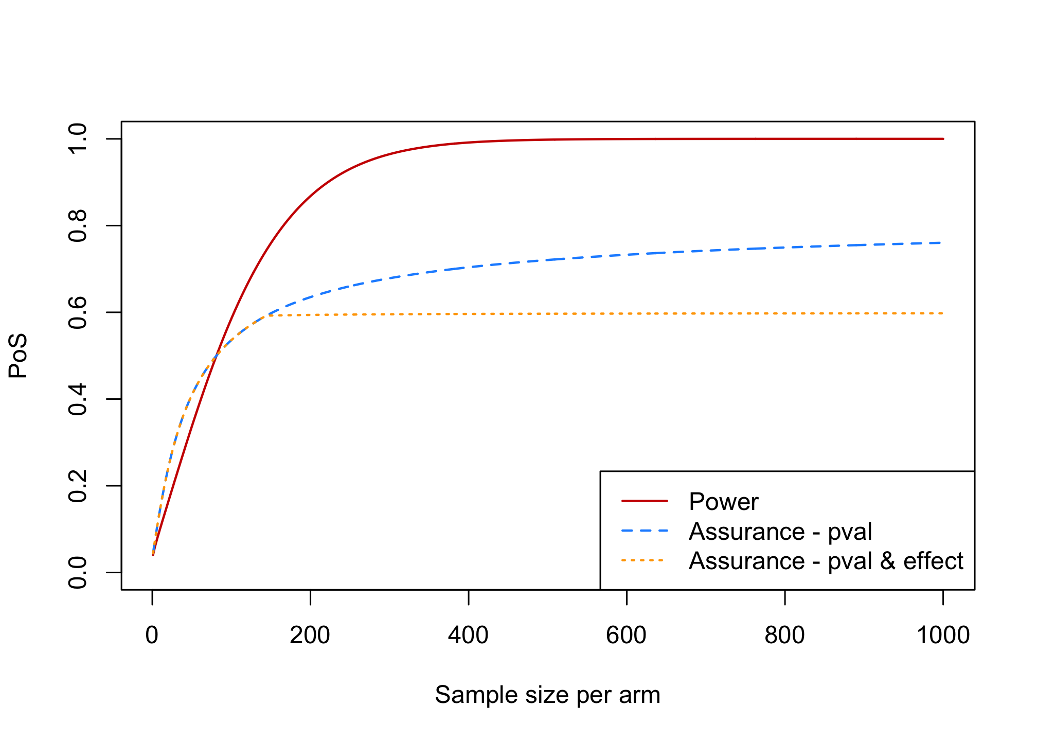
What is the upper bound for this version of assurance ?
assurance_fun_both(n = 10^8, mre = 1.5)## [1] 0.59870631 - pnorm(1.5, mean = 2, sd = 2)## [1] 0.5987063Also add to the plot a line for assurance where success is declared in case of a significant p-value for evaluating the null hypothesis that the effect equals 1.5
Hint: modify the formula from slide #31For this version of assurance, the critical value that needs to be exceeded is \(z_{1-\alpha}\tau+1.5\). Hence the formula for the assurance becomes:
\[P[\bar{y}_1 - \bar{y}_0 > z_{1-\alpha}\tau+1.5] = \Phi\left(\frac{-z_{1-\alpha}\tau-1.5 + \mu_{\delta}}{\sqrt{\sigma^2_{\delta}+\tau^2}}\right)\]assurance_fun_mre <- function(n, mre = 1.5, mu_delta = 2, sigma_delta = 2, sigma = 6.5, alpha = 0.025) { tau <- sigma * sqrt(2/n) asrc <- pnorm((-(qnorm(1 - alpha) * tau + mre) + mu_delta)/(sqrt(sigma_delta^2 + tau^2))) return(asrc) }n <- seq(1, 1000, 1) power_res <- sapply(n, power_fun) power_res_1.5 <- sapply(n, power_fun, delta = 1.5) assurance_res <- sapply(n, assurance_fun) assurance_res_1.5 <- sapply(n, assurance_fun_mre, mre = 1.5) plot(x = n, power_res, xlab = "Sample size per arm", ylab = "PoS", type = "l", col = "red3", ylim = c(0, 1), lwd = 1.5) lines(x = n, power_res_1.5, type = "l", col = "salmon", ylim = c(0, 1), lty = "dotted", lwd = 1.5) lines(x = n, assurance_res, type = "l", col = "dodgerblue", ylim = c(0, 1), lty = "dashed", lwd = 1.5) lines(x = n, assurance_res_1.5, type = "l", col = "purple", ylim = c(0, 1), lty = "dotdash", lwd = 1.5) legend("bottomright", legend = c("Power - H1: d>2", "Power - H1: d>1.5", "Assurance - pval H1: d≠0", "Assurance - pval H1: d>1.5"), col = c("red3", "salmon", "dodgerblue", "purple"), lty = c("solid", "dotted", "dashed", "dotdash"), lwd = 1.5)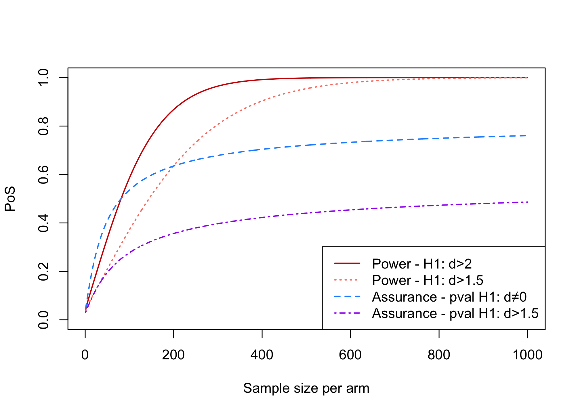
What is the upper bound for this version of assurance?
1 - pnorm(0, mean = 1.5, sd = 2)## [1] 0.7733726Which version of assurance do you prefer for the case study?
It is important that the success criterion for the trial matches the assurance.
For a large confirmatory trial, in practice a result is often considered acceptable when the p-value corresponding to the null hypothesis of no effect is significant and the point estimate is above a minimum relevant limit. This speaks in favor of the assurance from exercise 3.1. However, it would be important to evaluate whether this type of success criterion does not result in too many false positive results as the point estimate does not capture the variability around the estimate.
Assurance based on a p-value for the null hypothesis that the effect equals a minimum limit that needs to be exceeded could be appropriate. Drawbacks are that:
- it is hard to choose an appropriate effect size for the null hypothesis. In this example I chose the minimum relevant effect quite high for illustrative purposes. It is not easy to choose a good null hypothesis in this setting, as the effect in the null hypothesis needs to be large enough such that rejecting the null hypothesis implies that the effect of the drug is meaningful, but at the same time it should not include effect sizes that are meaningful as in those cases we would wish to conclude efficacy (reject the null hypothesis).
- designing a trial for such a null hypothesis results in much larger sample sizes such that the added benefit of such a more rigorous success criterion needs to be weighed against the extra resources required and the fact that more subjects need to be put at risk.
Bonus: what sample size would we need for the confirmatory trial if we wish to reject a null hypothesis that the effect equals \(1.5\) and we assume the effect is \(2\) under the alternative and we require \(90%\) power and wish to control the false positive rate at \(2.5%\) one-sided ?
Refer to slide #8:
we now have \(H_0: \mu_1-\mu_0 = 1.5\) and \(H_1:\mu_1-\mu_0 = 2\). Therefore we now need to ensure that \(1.5+z_{1-\alpha}\sigma\sqrt{2/n} = 2+z_{\beta}\sigma\sqrt{2/n}\) resulting in the same formula for the sample size, where \(\delta\) is replaced by \(\delta-1.5=2-1.5=0.5\).ssize <- 2 * 6.5^2 * (qnorm(1 - 0.025) + qnorm(1 - 0.1))^2/(0.5^2)
Exercise 4: the posterior conditional failure and success distributions for the case study
Write an function that returns the prior from Exercise 2 \(\pi(\delta)\) for a given \(\delta\).
Hint: use the functiondnormprior_delta <- function(delta, mu = 2, sigma = 2) { return(dnorm(delta, mean = mu, sd = sigma)) }Write an function that returns the likelihood \(P\left(\overline{y}_1-\overline{y}_0 > Z_{1-\alpha}\tau \lvert \delta\right)\) (i.e. the power) as a function of \(\delta\) for the confirmatory trial with a sample size of \(222\) patients per arm and a standard deviation of \(\sigma = 6.5\).
likelihood_success <- function(delta, n = 222, sigma = 6.5, alpha = 0.025) {
    tau <- sigma * sqrt(2/n)
    pwr <- pnorm(qnorm(alpha) + delta/tau)
    return(pwr)
}
Calculate the assurance for the confirmatory trial in case a sample size of \(222\) per arm is used and the success criterion is a significant p-value (you can re-use the result from Exercise 2 if you did it with a sample size of 222 per arm).
assurance_fun <- function(n = 222, mu_delta = 2, sigma_delta = 2, sigma = 6.5, alpha = 0.025) {
    tau <- sigma * sqrt(2/n)
    asrc <- pnorm((-qnorm(1 - alpha) * tau + mu_delta)/(sqrt(sigma_delta^2 + tau^2)))
    return(asrc)
}
assurance_222constant <- assurance_fun()
Use the results from steps 1-3 to create a plot of the posterior conditional success distribution.
posterior_csd <- function(delta, samplesize = 222) {
    prior_delta(delta) * likelihood_success(delta, n = samplesize)/assurance_fun(n = samplesize)
}

d <- seq(-5, 15, 0.1)
post_csd_res <- sapply(d, posterior_csd)

plot(x = d, post_csd_res, xlab = expression(delta), ylab = "Posterior conditional success distribution",
    type = "l", col = "darkgreen", lwd = 2)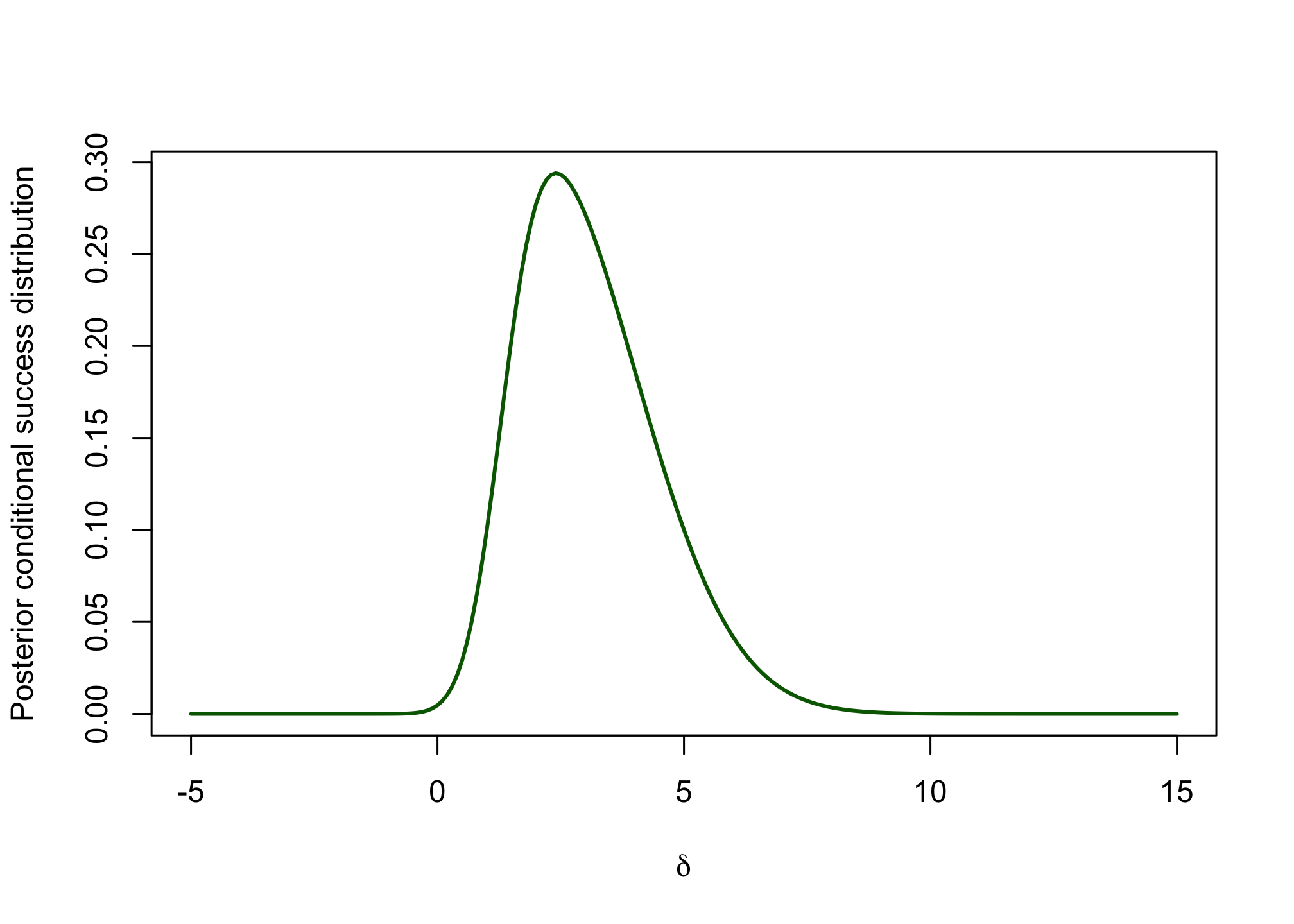
Similarly, derive the posterior conditional failure distribution and add it to the plot.
posterior_csf <- function(delta, samplesize = 222) {
    prior_delta(delta) * (1 - likelihood_success(delta, n = samplesize))/(1 - assurance_fun(n = samplesize))
}

post_csd_res <- sapply(d, posterior_csd)
post_csf_res <- sapply(d, posterior_csf)

plot(x = d, post_csd_res, xlab = expression(delta), ylab = "Posterior conditional distribution",
    type = "l", col = "darkgreen", lwd = 2, xlim = c(-5, 15), ylim = c(0, 0.6), main = "Sample-size = 222")
lines(x = d, post_csf_res, xlab = expression(delta), type = "l", col = "red", lwd = 2,
    lty = 2)
abline(v = 1.45, lty = 3)
legend("topright", legend = c("Success", "Failure"), col = c("darkgreen", "red"),
    lty = c("solid", "dashed"), lwd = 2)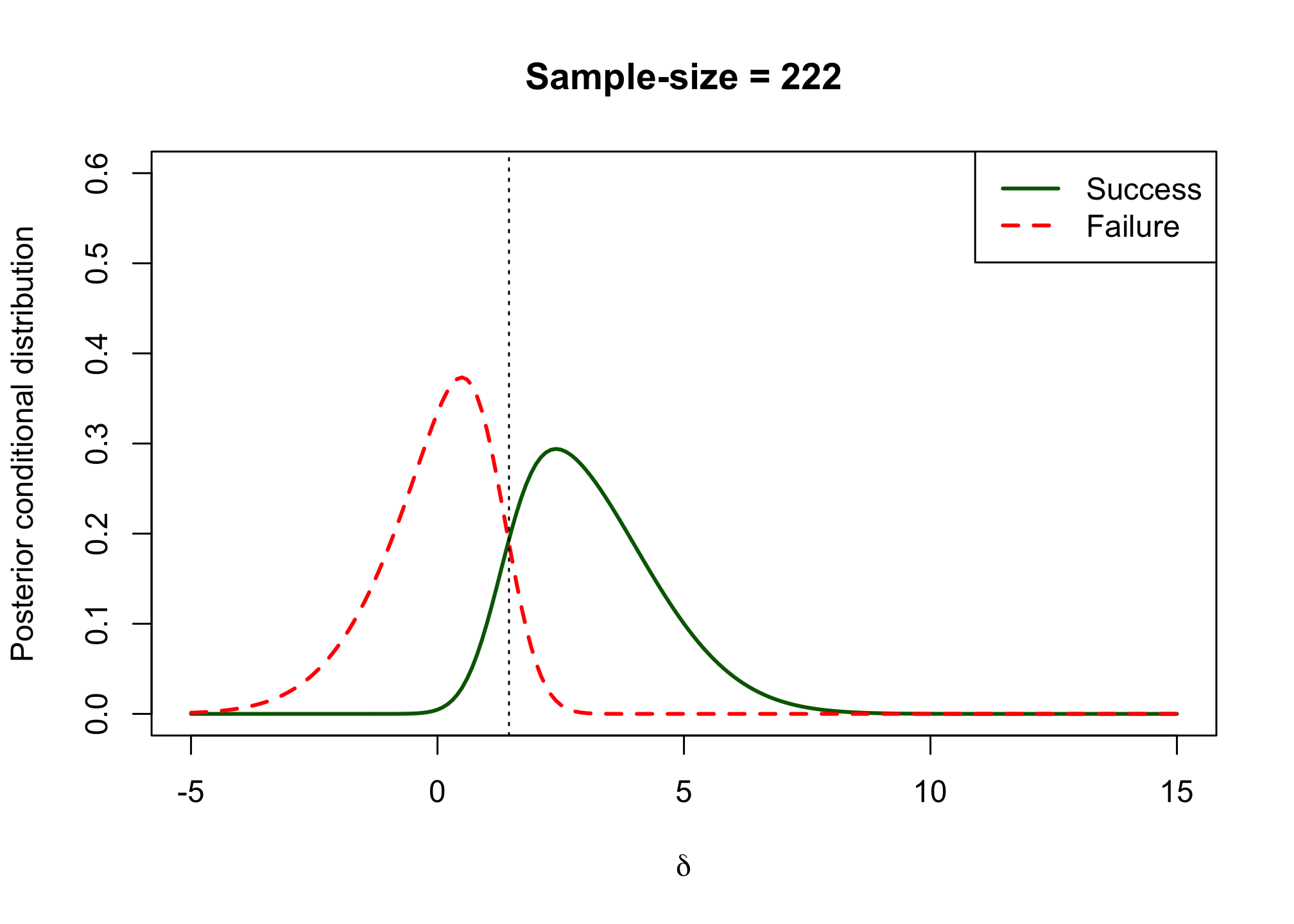
Are you satisfied with the proposed design in its ability to distinguish between a drug that works and a drug that doesn’t work?
Ideally the overlap between the two functions is small. In this case we can see that some successes are concluded when the true effect is below \(1.5\) and some failures are concluded despite the effect being above \(1.5\). However, the overlap between the two functions is not very large and may be acceptable.
post_csd_res <- sapply(d, posterior_csd, samplesize = 2000)
post_csf_res <- sapply(d, posterior_csf, samplesize = 2000)

plot(x = d, post_csd_res, xlab = expression(delta), ylab = "Posterior conditional distribution",
    type = "l", col = "darkgreen", lwd = 2, xlim = c(-5, 15), ylim = c(0, 0.6), main = "Sample-size = 2000")
lines(x = d, post_csf_res, xlab = expression(delta), type = "l", col = "red", lwd = 2,
    lty = 2)
abline(v = 0.6, lty = 3)
legend("topright", legend = c("Success", "Failure"), col = c("darkgreen", "red"),
    lty = c("solid", "dashed"), lwd = 2)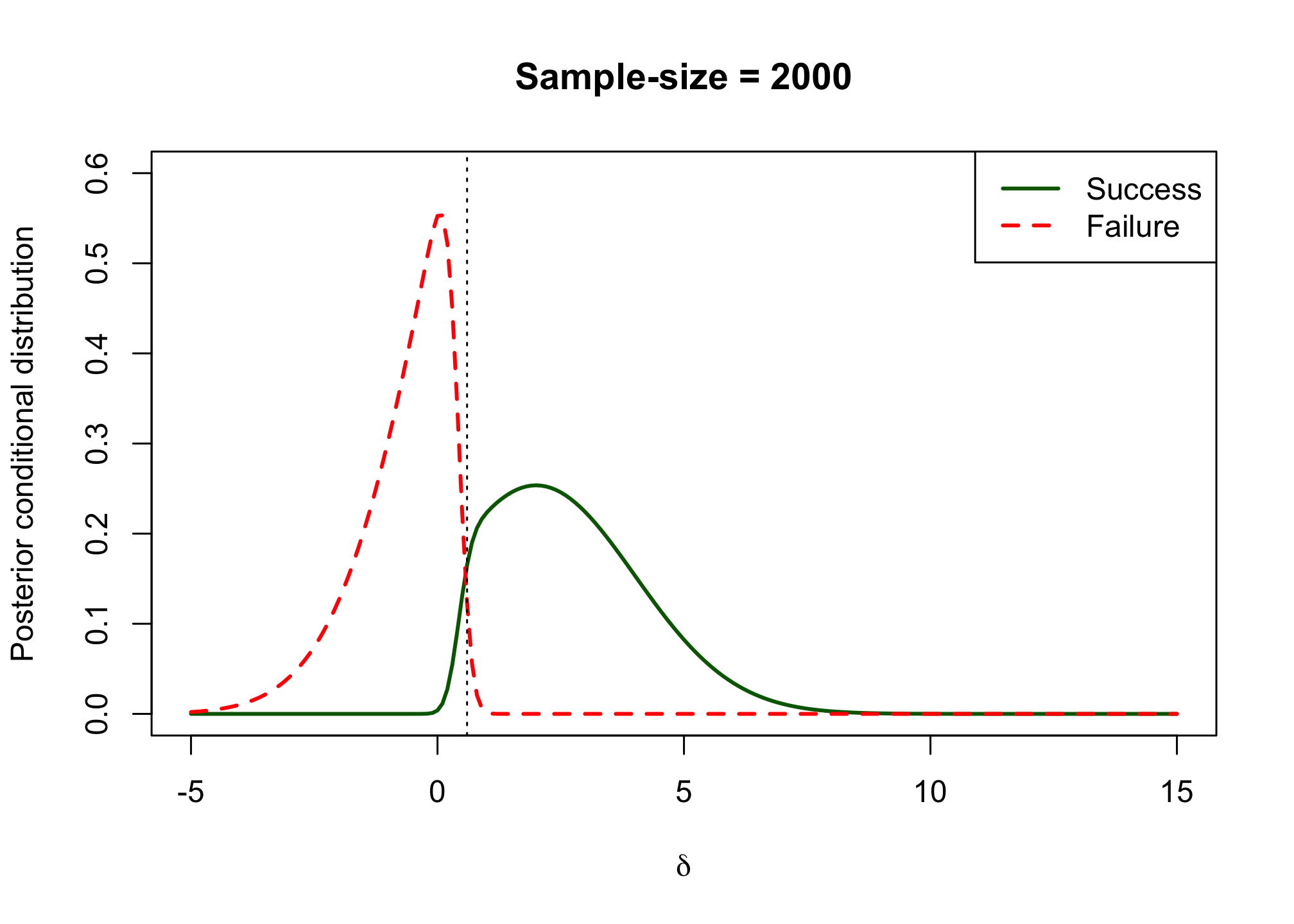
The code below gives the posterior conditional success and failure distributions for assurance when success is declared if the point estimate is above the minimum relevant effect. The curves are quite similar, but shifted slightly to the right.
pwr2 <- function(sigma, delta, alpha, n, mre) {
    pnorm((-max(mre, qnorm(1 - alpha) * sigma * sqrt(2/n)) + delta)/(sigma * sqrt(2/n)))
}

pcsd2 <- function(delta, mu_delta = 2, sigma_delta = 2, sigma = 6.5, alpha = 0.025,
    beta = 0.1, n = 222, mre = 1.5) {
    prior_delta(delta, mu_delta, sigma_delta) * pwr2(delta, sigma = sigma, alpha = alpha,
        n = n, mre = mre)/assurance_fun_both(sigma = sigma, alpha = alpha, n = n,
        mu_delta = mu_delta, sigma_delta = sigma_delta, mre = mre)
}

pcfd2 <- function(delta, mu_delta = 2, sigma_delta = 2, sigma = 6.5, alpha = 0.025,
    beta = 0.1, n = 222, mre = 1.5) {
    prior_delta(delta, mu_delta, sigma_delta) * (1 - pwr2(delta, sigma = sigma, alpha = alpha,
        n = n, mre = mre))/(1 - assurance_fun_both(sigma = sigma, alpha = alpha,
        n = n, mu_delta = mu_delta, sigma_delta = sigma_delta, mre = mre))
}

success_res2 <- sapply(d, pcsd2)
failure_res2 <- sapply(d, pcfd2)

plot(d, success_res2, type = "l", col = "darkgreen", lwd = 2, xlab = "delta", ylab = "Density",
    ylim = c(0, 0.5))
lines(d, failure_res2, col = "red", lwd = 2)
abline(v = 1.45, lty = 3)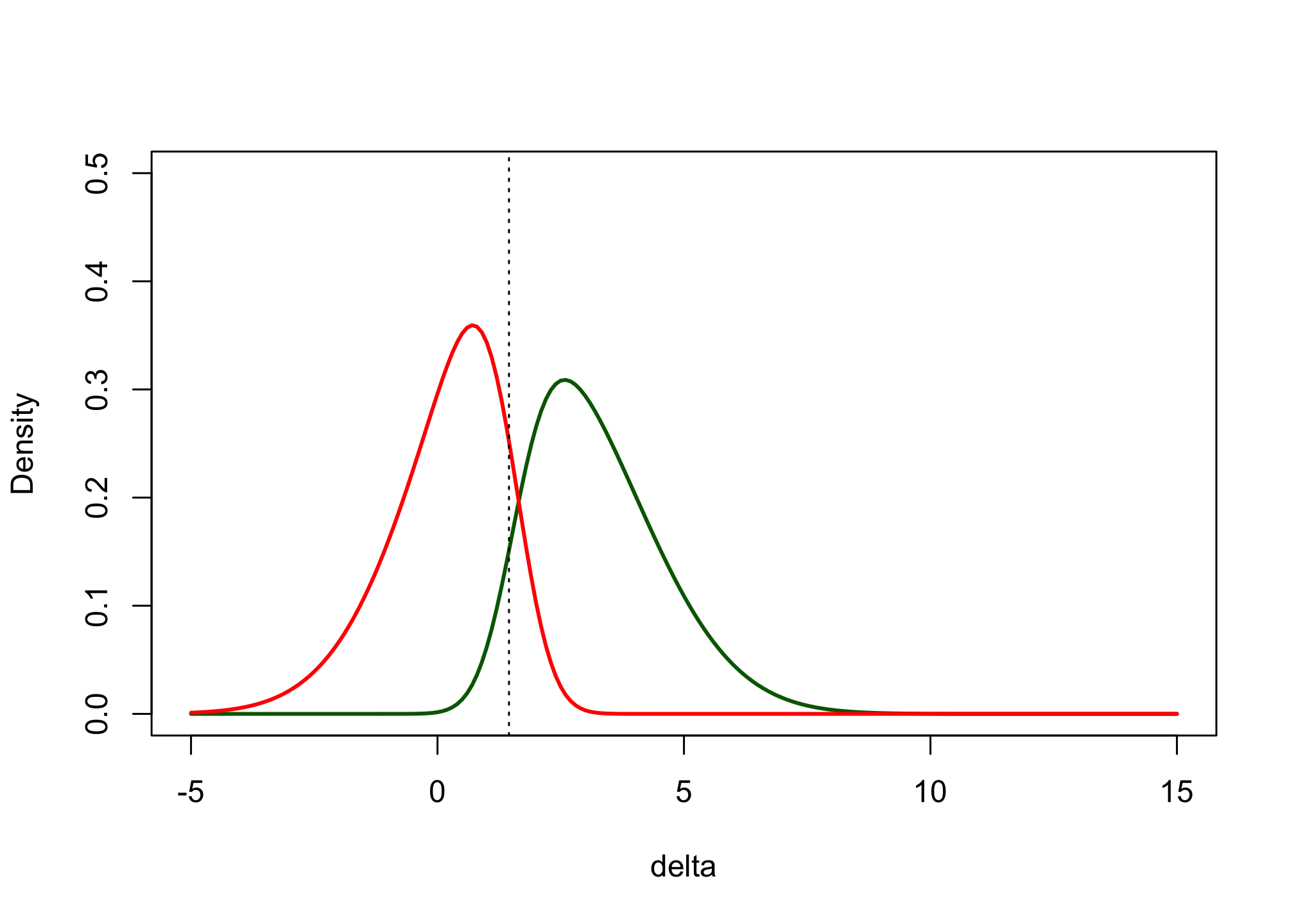
Exercise 5
Compute the probability of a true success for the confirmatory trial where a significant p-value is considered the criterion for success (for the null hypothesis of no effect).
Hint: use the functionpmvnormfrom the packagemvtnormlibrary(mvtnorm) tau <- 6.5 * sqrt(2/222) sigma_prior <- 2 cmat <- matrix(c(tau^2 + sigma_prior^2, sigma_prior^2, sigma_prior^2, sigma_prior^2), nrow = 2, byrow = T) res <- pmvnorm(lower = c(qnorm(0.975) * tau, 0), upper = Inf, mean = c(2, 2), sigma = cmat) res## [1] 0.6465897 ## attr(,"error") ## [1] 1e-15 ## attr(,"msg") ## [1] "Normal Completion"The probability of a true success equals \(0.6466\). This is very similar to the assurance calculated earlier \(0.6472\).
The difference is small because the power for an effect below \(0\) is at most \(2.5\%\) and the prior probability of an effect below \(0\) is small (0.159).
Compare this probability to the assurance you calculated earlier.
assurance_both_222constant <- assurance_fun_both(sigma = 6.5, alpha = 0.025, n = 222,
    mu_delta = 2, sigma_delta = 2, mre = 1.5)
assurance_both_222constant
## [1] 0.5944054res2 <- pmvnorm(lower = c(1.5, 1.5), upper = Inf, mean = c(2, 2), sigma = cmat)The probability of a true success equals \(0.5503\). This is a bit lower than the assurance using a success criterion requiring a significant p-value and a point estimate above 1.5, which is \(0.5944\).
Compute the probability of a true success for the confirmatory trial where a significant p-value as well as a point estimate above 1.5 is considered the criterion for success.
Compare your result from step 3 to the same version of assurance where we do not require a true success.